 with respect to
 .
This is the original Axiom book from 1992 with title “AXIOM—The Scientific Computation System” by Jenks and Sutor in its adaptation for the FriCAS fork of the Axiom source code.
It counts as the official version for the FriCAS project.
The original sources (including the text and scripts) for this book were released in 2002, under the modified BSD license that is found in the file LICENSE.txt in the source code repository of FriCAS.
e0b2ccbb1e222d5a0fa8765205e099db6f91fa40
Since this book is a moving target, each part of its generation is automated. In particular, the output of FriCAS commands (including their typesetting in LaTeX) is automated. However, that sometimes means that you see boxes with output that does not fit the width of the page. We use the breqn LaTeX package to break equations appropriately. Unfortunately, that does not always work nicely.
If you find other inaccuracies, please report them to the mailing list fricas-devel@googlegroups.com.
The book is an effort of quite a number of people. The original Axiom book lists the following people as authors: Manuel Bronstein, William H. Burge, Timothy P. Daly, Patrizia Gianni, Johannes Grabmeier, Scott C. Morrison, Jonathan M. Steinbach, Robert S. Sutor, Barry M. Trager, Stephen M. Watt, Richard D. Jenks, Clifton J. Williamson.
Since FriCAS has been forked from the Axiom project, there have been a number of contributions and corrections by Martin Baker, Riccardo Guida, Waldek Hebisch, Ralf Hemmecke, Qian Yun.
Welcome to the world of FriCAS. We call FriCAS a scientific computation system: a self-contained toolbox designed to meet your scientific programming needs, from symbolics, to numerics, to graphics.
This introduction is a quick overview of what FriCAS offers.
FriCAS provides a wide range of simple commands for symbolic mathematical problem solving. Do you need to solve an equation, to expand a series, or to obtain an integral? If so, just ask FriCAS to do it.
Integrate with respect to .
integrate(1/(x^3 * (a+b*x)^(1/3)),x)
Union(Expression(Integer), ...)
FriCAS provides state-of-the-art algebraic machinery to handle your most advanced symbolic problems. For example, FriCAS’s integrator gives you the answer when an answer exists. If one does not, it provides a proof that there is no answer. Integration is just one of a multitude of symbolic operations that FriCAS provides.
FriCAS has a numerical library that includes operations for linear algebra, solution of equations, and special functions. For many of these operations, you can select any number of floating point digits to be carried out in the computation.
Solve  to 49 digits of accuracy.
digits(49); solve(x^49-49*x^4+9 = 0,1.e-49)
List(Equation(Polynomial(Float)))
The output of a computation can be converted to FORTRAN to be used in a later numerical computation. Besides floating point numbers, FriCAS provides literally dozens of kinds of numbers to compute with. These range from various kinds of integers, to fractions, complex numbers, quaternions, continued fractions, and to numbers represented with an arbitrary base.
What is 10 to the  power in base
32?
radix(10^100,32)
You may often want to visualize a symbolic formula or draw a graph from a set of numerical values. To do this, you can call upon the FriCAS graphics capability.
Draw  for
 .
draw(5*besselJ(0,sqrt(x^2+y^2)), x=-20..20, y=-20..20)
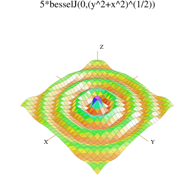
Graphs in FriCAS are interactive objects you can manipulate with your mouse. Just click on the graph, and a control panel pops up. Using the mouse and the control panel, you can translate, rotate, zoom, change the coloring, lighting, shading, and perspective on the picture. You can also generate a PostScript copy of your graph to produce hard-copy output.
HyperDoc presents you with windows on the world of FriCAS, offering on-line help, examples, tutorials, a browser, and reference material. HyperDoc gives you on-line access to this book in a “hypertext” format. Words that appear in a different font (for example, Matrix, factor, and category) are generally mouse-active; if you click on one with your mouse, HyperDoc shows you a new window for that word.
As another example of a HyperDoc facility, suppose that you want to compute the roots of  to
 digits (as in our previous example) and you don’t know how to tell FriCAS to do this. The “basic
command” facility of HyperDoc leads the way. Through the series of HyperDoc windows shown in Figure 0.4
and the specified mouse clicks, you and HyperDoc generate the correct command to issue to compute the
answer.
Computing the roots of 
FriCAS’s interactive programming language lets you define your own functions. A simple example of a user-defined function is one that computes the successive Legendre polynomials. FriCAS lets you define these polynomials in a piece-wise way.
The first Legendre polynomial.
p(0) == 1
The second Legendre polynomial.
p(1) == x
The  Legendre polynomial for
 .
p(n) == ((2*n-1)*x*p(n-1) - (n-1) * p(n-2))/n
In addition to letting you define simple functions like this, the interactive language can be used to create entire application packages. All the graphs in the FriCAS Images section in the center of the book, for example, were created by programs written in the interactive language.
The above definitions for p do no computation—they simply tell FriCAS how to compute p(k)
for some positive integer k. To actually get a value of a Legendre polynomial, you ask for it.
What is the tenth Legendre polynomial?
p(10)
Compiling function p with type Integer -> Polynomial(Fraction(Integer))
Compiling function p as a recurrence relation.
FriCAS applies the above pieces for p to obtain the value of p(10). But it does more: it creates an optimized,
compiled function for p. The function is formed by putting the pieces together into a single piece of code. By
compiled, we mean that the function is translated into basic machine-code. By optimized, we mean that
certain transformations are performed on that code to make it run faster. For p, FriCAS actually translates
the original definition that is recursive (one that calls itself) to one that is iterative (one that consists of a
simple loop).
What is the coefficient of  in
p(90)?
coefficient(p(90),x,90)
In general, a user function is type-analyzed and compiled on first use. Later, if you use it with a different kind of object, the function is recompiled if necessary.
A variety of data structures are available for interactive use. These include strings, lists, vectors, sets, multisets, and hash tables. A particularly useful structure for interactive use is the infinite stream:
Create the infinite stream of derivatives of Legendre polynomials
[D(p(i),x) for i in 1..]
Stream(Polynomial(Fraction(Integer)))
Streams display only a few of their initial elements. Otherwise, they are “lazy”: they only compute elements when you ask for them.
Data structures are an important component for building application software. Advanced users can represent data for applications in optimal fashion. In all, FriCAS offers over forty kinds of aggregate data structures, ranging from mutable structures (such as cyclic lists and flexible arrays) to storage efficient structures (such as bit vectors). As an example, streams are used as the internal data structure for power series.
What is the series expansion of  about
 ?
series(log(cot(x)),x = %pi/2)
GeneralUnivariatePowerSeries(Expression(Integer), x, \%pi/2)
Series and streams make no attempt to compute all their elements! Rather, they stand ready to deliver elements on demand.
What is the coefficient of the  term of this series?
coefficient(%,50)
FriCAS also has many kinds of mathematical structures. These range from simple ones (like polynomials and matrices) to more esoteric ones (like ideals and Clifford algebras). Most structures allow the construction of arbitrarily complicated “types.”
Even a simple input expression can result in a type with several levels.
matrix [[x + %i,0], [1,-2]]
Matrix(Polynomial(Complex(Integer)))
The FriCAS interpreter builds types in response to user input. Often, the type of the result is changed in order to be applicable to an operation.
The inverse operation requires that elements of the above matrices are fractions.
inverse(%)
Union(Matrix(Fraction(Polynomial(Complex(Integer)))), ...)
A convenient facility for symbolic computation is “pattern matching.” Suppose you have a trigonometric
expression and you want to transform it to some equivalent form. Use a rule command to describe the
transformation rules you need. Then give the rules a name and apply that name as a function to your
trigonometric expression.
Introduce two rewrite rules.
sinCosExpandRules := rule sin(x+y) == sin(x)*cos(y) + sin(y)*cos(x) cos(x+y) == cos(x)*cos(y) - sin(x)*sin(y) sin(2*x) == 2*sin(x)*cos(x) cos(2*x) == cos(x)^2 - sin(x)^2
Ruleset(Integer, Integer, Expression(Integer))
Apply the rules to a simple trigonometric expression.
sinCosExpandRules(sin(a+2*b+c))
Using input files, you can create your own library of transformation rules relevant to your applications, then selectively apply the rules you need.
All components of the FriCAS algebra library are written in the FriCAS library language. This language is similar to the interactive language except for protocols that authors are obliged to follow. The library language permits you to write “polymorphic algorithms,” algorithms defined to work in their most natural settings and over a variety of types.
Define a system of polynomial equations S.
S := [3*x^3 + y + 1 = 0,y^2 = 4]
List(Equation(Polynomial(Integer))) Solve the system S using rational number arithmetic and 30 digits of accuracy.
digits(30); solve(S,1/10^30)
List(List(Equation(Polynomial(Fraction(Integer))))) Solve S with the solutions expressed in radicals.
radicalSolve(S)
List(List(Equation(Expression(Integer))))
While these solutions look very different, the results were produced by the same internal algorithm! The internal algorithm actually works with equations over any “field.” Examples of fields are the rational numbers, floating point numbers, rational functions, power series, and general expressions involving radicals.
Users and system developers alike can augment the FriCAS library, all using one common language. Library code, like interpreter code, is compiled into machine binary code for run-time efficiency.
Using this language, you can create new computational types and new algorithmic packages. All library code is polymorphic, described in terms of a database of algebraic properties. By following the language protocols, there is an automatic, guaranteed interaction between your code and that of colleagues and system implementers.
FriCAS has both an interactive language for user interactions and a programming language for building library modules. Like Modula 2, PASCAL, FORTRAN, and Ada, the programming language emphasizes strict type-checking. Unlike these languages, types in FriCAS are dynamic objects: they are created at run-time in response to user commands.
Here is the idea of the FriCAS programming language in a nutshell. FriCAS types range from algebraic ones (like polynomials, matrices, and power series) to data structures (like lists, dictionaries, and input files). Types combine in any meaningful way. You can build polynomials of matrices, matrices of polynomials of power series, hash tables with symbolic keys and rational function entries, and so on.
Categories define algebraic properties to ensure mathematical correctness. They ensure, for example, that matrices of polynomials are OK, but matrices of input files are not. Through categories, programs can discover that polynomials of continued fractions have a commutative multiplication whereas polynomials of matrices do not.
Categories allow algorithms to be defined in their most natural setting. For example, an algorithm can be defined to solve polynomial equations over any field. Likewise a greatest common divisor can compute the “gcd” of two elements from any Euclidean domain. Categories foil attempts to compute meaningless “gcds”, for example, of two hashtables. Categories also enable algorithms to be compiled into machine code that can be run with arbitrary types.
The FriCAS interactive language is oriented towards ease-of-use. The FriCAS interpreter uses type-inferencing to deduce the type of an object from user input. Type declarations can generally be omitted for common types in the interactive language.
So much for the nutshell. Here are these basic ideas described by ten design principles:
Basic types are called domains of computation, or, simply, domains. Domains are defined by FriCAS programs of the form:
Name(...): Exports == Implementation
Each domain has a capitalized Name that is used to refer to the class of its members. For example, Integer denotes “the class of integers,” Float, “the class of floating point numbers,” and String, “the class of strings.”
The “...” part following Name lists zero or more parameters to the constructor. Some basic ones like Integer take no parameters. Others, like Matrix, Polynomial and List, take a single parameter that again must be a domain. For example, Matrix(Integer) denotes “matrices over the integers,” Polynomial (Float) denotes “polynomial with floating point coefficients,” and List (Matrix (Polynomial (Integer))) denotes “lists of matrices of polynomials over the integers.” There is no restriction on the number or type of parameters of a domain constructor.
The Exports part specifies operations for creating and manipulating objects of the domain. For example, type
Integer exports constants 0 and 1, and operations +, -, and *. While these operations are common, others
such as odd? and bit? are not.
The Implementation part defines functions that implement the exported operations of the domain. These functions are frequently described in terms of another lower-level domain used to represent the objects of the domain.
Every FriCAS object belongs to a unique domain. The domain of an object is also called its type. Thus the
integer 7 has type Integer and the string "daniel" has type String.
The type of an object, however, is not unique. The type of integer 7 is not only Integer but
NonNegativeInteger, PositiveInteger, and possibly, in general, any other “subdomain” of the domain
Integer. A subdomain is a domain with a “membership predicate”. PositiveInteger is a subdomain of
Integer with the predicate “is the integer > 0?”.
Subdomains with names are defined by abstract datatype programs similar to those for domains. The Export part of a subdomain, however, must list a subset of the exports of the domain. The Implementation part optionally gives special definitions for subdomain objects.
Domain and subdomains in FriCAS are themselves objects that have types. The type of a domain or subdomain is called a category. Categories are described by programs of the form:
Name(...): Category == Exports
The type of every category is the distinguished symbol Category. The category Name is used to designate the class of domains of that type. For example, category Ring designates the class of all rings. Like domains, categories can take zero or more parameters as indicated by the “...” part following Name. Two examples are Module(R) and MatrixCategory(R,Row,Col).
The Exports part defines a set of operations. For example, Ring exports the operations 0, 1, +, -, and *.
Many algebraic domains such as Integer and Polynomial (Float) are rings. String and List (R) (for any
domain R) are not.
Categories serve to ensure the type-correctness. The definition of matrices states Matrix(R: Ring) requiring
its single parameter R to be a ring. Thus a “matrix of polynomials” is allowed, but “matrix of lists” is
not.
All operations have prescribed source and target types. Types can be denoted by symbols that stand for
domains, called “symbolic domains.” The following lines of FriCAS code use a symbolic domain
R:
R: Ring power: (R, NonNegativeInteger): R -> R power(x, n) == x ** n
Line 1 declares the symbol R to be a ring. Line 2 declares the type of power in terms of R. From the definition
on line 3, power(3,2) produces 9 for x = 3 and R = Integer. Also, power(3.0,2) produces 9.0 for x = 3.0 and
R = Float. power("oxford",2) however fails since "oxford" has type String which is not a
ring.
Using symbolic domains, algorithms can be defined in their most natural or general setting.
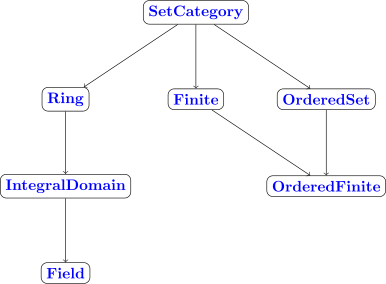
Categories form hierarchies (technically, directed-acyclic graphs). A simplified hierarchical world of algebraic categories is shown below in Figure 0.10. At the top of this world is SetCategory, the class of algebraic sets. The notions of parents, ancestors, and descendants is clear. Thus ordered sets (domains of category OrderedSet) and rings are also algebraic sets. Likewise, fields and integral domains are rings and algebraic sets. However fields and integral domains are not ordered sets.
A category designates a class of domains. Which domains? You might think that Ring designates the class of
all domains that export 0, 1, +, -, and *. But this is not so. Each domain must assert which categories it
belongs to.
The Export part of the definition for Integer reads, for example:
Join(OrderedSet, IntegralDomain, ...) with ...
This definition asserts that Integer is both an ordered set and an integral domain. In fact, Integer does not
explicitly export constants 0 and 1 and operations +, - and * at all: it inherits them all from Ring! Since
IntegralDomain is a descendant of Ring, Integer is therefore also a ring.
Assertions can be conditional. For example, Complex(R) defines its exports by:
Ring with ... if R has Field then Field ...
Thus Complex(Float) is a field but Complex(Integer) is not since Integer is not a field.
You may wonder: “Why not simply let the set of operations determine whether a domain belongs to a given
category?”. FriCAS allows operation names (for example, norm) to have very different meanings in different
contexts. The meaning of an operation in FriCAS is determined by context. By associating operations with
categories, operation names can be reused whenever appropriate or convenient to do so. As a simple example,
the operation < might be used to denote lexicographic-comparison in an algorithm. However, it is wrong to
use the same < with this definition of absolute-value: abs(x) == if x < 0 then -x else x. Such a
definition for abs in FriCAS is protected by context: argument x is required to be a member of a domain of
category OrderedSet.
In FriCAS, facilities for symbolic integration, solution of equations, and the like are placed in “packages”. A package is a special kind of domain: one whose exported operations depend solely on the parameters of the constructor and/or explicit domains.
If you want to use FriCAS, for example, to define some algorithms for solving equations of polynomials over
an arbitrary field F, you can do so with a package of the form:
MySolve(F: Field): Exports == Implementation
where Exports specifies the solve operations you wish to export and Implementation defines functions for
implementing your algorithms. Once FriCAS has compiled your package, your algorithms can then be used for
any F: floating-point numbers, rational numbers, complex rational functions, and power series, to name a
few.
The FriCAS interpreter reads user input then builds whatever types it needs to perform the indicated computations. For example, to create the matrix
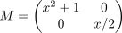
the interpreter first loads the modules Matrix, Polynomial, Fraction, and Integer from the library, then builds the domain tower “matrices of polynomials of rational numbers (fractions of integers)”.
Once a domain tower is built, computation proceeds by calling operations down the tower. For example,
suppose that the user asks to square the above matrix. To do this, the function * from Matrix is passed M
to compute M * M. The function is also passed an environment containing R that, in this case, is
Polynomial (Fraction (Integer)). This results in the successive calling of the * operations from
Polynomial, then from Fraction, and then finally from Integer before a result is passed back up the
tower.
Categories play a policing role in the building of domains. Because the argument of Matrix is required to be a ring, FriCAS will not build nonsensical types such as “matrices of input files”.
FriCAS programs are statically compiled to machine code, then placed into library modules. Categories provide an important role in obtaining efficient object code by enabling:
R”, for
instance, can be open-coded even though R is unknown).
Users and system implementers alike use the FriCAS language to add facilities to the FriCAS library. The entire FriCAS library is in fact written in the FriCAS source code and available for user modification and/or extension.
FriCAS’s use of abstract datatypes clearly separates the exports of a domain (what operations are defined) from its implementation (how the objects are represented and operations are defined). Users of a domain can thus only create and manipulate objects through these exported operations. This allows implementers to “remove and replace” parts of the library safely by newly upgraded (and, we hope, correct) implementations without consequence to its users.
Categories protect names by context, making the same names available for use in other contexts. Categories also provide for code-economy. Algorithms can be parameterized categorically to characterize their correct and most general context. Once compiled, the same machine code is applicable in all such contexts.
Finally, FriCAS provides an automatic, guaranteed interaction between new and old code. For example:
These are the key ideas. For further information, we particularly recommend your reading chapters 11, 12, and 13, where these ideas are explained in greater detail.
Welcome to the FriCAS environment for interactive computation and problem solving. Consider this chapter a brief, whirlwind tour of the FriCAS world. We introduce you to FriCAS’s graphics and the FriCAS language. Then we give a sampling of the large variety of facilities in the FriCAS system, ranging from the various kinds of numbers, to data types (like lists, arrays, and sets) and mathematical objects (like matrices, integrals, and differential equations). We conclude with the discussion of system commands and an interactive “undo.”
Before embarking on the tour, we need to brief those readers working interactively with FriCAS on some details. Others can skip immediately to Section 1.2 on page 37.
You need to know how to start the FriCAS system and how to stop it. We assume that FriCAS has been correctly installed on your machine (as described in another FriCAS document).
To begin using FriCAS, issue the command fricas to the operating system shell. There is a brief pause, some start-up messages, and then one or more windows appear.
If you are not running FriCAS under the X Window System, there is only one window (the console). At the lower left of the screen there is a prompt that looks like
(1) ->
When you want to enter input to FriCAS, you do so on the same line after the prompt. The “1” in “(1)” is the computation step number and is incremented after you enter FriCAS statements. Note, however, that a system command such as )clear all may change the step number in other ways. We talk about step numbers more when we discuss system commands and the workspace history facility.
If you are running FriCAS under the X Window System, there may be two windows: the console window (as just described) and the HyperDoc main menu. HyperDoc is a multiple-window hypertext system that lets you view FriCAS documentation and examples on-line, execute FriCAS expressions, and generate graphics. If you are in a graphical windowing environment, it is usually started automatically when FriCAS begins. If it is not running, issue )hd to start it. We discuss the basics of HyperDoc in Chapter 3.
To interrupt an FriCAS computation, hold down the Ctrl (control) key and press c. This brings you back to the FriCAS prompt.
To exit from FriCAS, move to the console window, type )quit at the input prompt and press the Enter key. You will probably be prompted with the following message:
Please enter y or yes if you really want to leave the
interactive environment and return to the operating system
You should respond yes, for example, to exit FriCAS.
We are purposely vague in describing exactly what your screen looks like or what messages FriCAS displays. FriCAS runs on a number of different machines, operating systems and window environments, and these differences all affect the physical look of the system. You can also change the way that FriCAS behaves via system commands described later in this chapter and in Appendix 15.4.10. System commands are special commands, like )set, that begin with a closing parenthesis and are used to change your environment. For example, you can set a system variable so that you are not prompted for confirmation when you want to leave FriCAS.
If you are using FriCAS under the X Window System, the Clef command line editor is probably available and installed. With this editor you can recall previous lines with the up and down arrow keys.
To move forward and backward on a line, use the right and left arrows. You can use the Insert key to toggle insert mode on or off. When you are in insert mode, the cursor appears as a large block and if you type anything, the characters are inserted into the line without deleting the previous ones.
If you press the Home key, the cursor moves to the beginning of the line and if you press the End key, the cursor moves to the end of the line. Pressing Ctrl–End deletes all the text from the cursor to the end of the line.
Clef also provides FriCAS operation name completion for a limited set of operations. If you enter a few letters and then press the Tab key, Clef tries to use those letters as the prefix of an FriCAS operation name. If a name appears and it is not what you want, press Tab again to see another name.
You are ready to begin your journey into the world of FriCAS. Proceed to the first stop.
In this book we have followed these typographical conventions:
inc(x)== x + 1.

This book contains over 2500 examples of FriCAS input and output. All examples were run through FriCAS and their output was created in LaTeX form for this book by the FriCAS FormatLaTeX package.
The FriCAS language is a rich language for performing interactive computations and for building components of the FriCAS library. Here we present only some basic aspects of the language that you need to know for the rest of this chapter. Our discussion here is intentionally informal, with details unveiled on an “as needed” basis. For more information on a particular construct, we suggest you consult the index at the back of the book.
For arithmetic expressions, use the + and - operators as in mathematics. Use * for multiplication, and ^ for exponentiation. To create a fraction, use /. When an expression contains several operators, those of highest precedence are evaluated first. For arithmetic operators, ^ has highest precedence, * and / have the next highest precedence, and + and - have the lowest precedence.
FriCAS puts implicit parentheses around operations of higher precedence, and groups those of equal precedence from left to right.
1 + 2 - 3 / 4 * 3 ^ 2 - 1
Fraction(Integer) The above expression is equivalent to this.
((1 + 2) - ((3 / 4) * (3 ^ 2))) - 1
Fraction(Integer) If an expression contains subexpressions enclosed in parentheses, the parenthesized subexpressions are evaluated first (from left to right, from inside out).
1 + 2 - 3/ (4 * 3 ^ (2 - 1))
Use the percent sign (“%”) to refer to the last result. Also, use “%%” to refer to previous results. %%(-1)
is equivalent to “%”, %%(-2) returns the next to the last result, and so on. %%(1) returns the
result from step number 1, %%(2) returns the result from step number 2, and so on. %%(0) is not
defined.
This is ten to the tenth power.
10 ^ 10
PositiveInteger This is the last result minus one.
% - 1
PositiveInteger This is the last result.
%%(-1)
PositiveInteger This is the result from step number 1.
%%(1)
Everything in FriCAS has a type. The type determines what operations you can perform on an object and how the object can be used. An entire chapter of this book (Chapter 2) is dedicated to the interactive use of types. Several of the final chapters discuss how types are built and how they are organized in the FriCAS library.
Positive integers are given type PositiveInteger.
8
PositiveInteger Negative ones are given type Integer. This fine distinction is helpful to the FriCAS interpreter.
-8
Integer Here a positive integer exponent gives a polynomial result.
x^8
Polynomial(Integer) Here a negative integer exponent produces a fraction.
x^(-8)
A symbol is a literal used for the input of things like the “variables” in polynomials and power series.
We use the three symbols x, y, and z in entering this polynomial.
(x - y*z)^2
Polynomial(Integer) A symbol has a name beginning with an uppercase or lowercase alphabetic character,
“%”, or “!”. Successive characters (if any) can be any of the above, digits, or “?”. Case is distinguished: the
symbol points is different from the symbol Points.
A symbol can also be used in FriCAS as a variable. A variable refers to a value. To assign a value to a variable, the operator “:=” is used.1 A variable initially has no restrictions on the kinds of values to which it can refer.
This assignment gives the value 4 (an integer) to a variable named x.
x := 4
PositiveInteger This gives the value z + 3/5 (a polynomial) to x.
x := z + 3/5
Polynomial(Fraction(Integer)) To restrict the types of objects that can be assigned to a variable, use a declaration
y : Integer
After a variable is declared to be of some type, only values of that type can be assigned to that variable.
y := 89
Integer The declaration for y forces values assigned to y to be converted to integer values.
y := sin %pi
Integer If no such conversion is possible, FriCAS refuses to assign a value to y.
y := 2/3
Cannot convert right-hand side of assignment 2 - 3 to an object of the type Integer of the left-hand side.
A type declaration can also be given together with an assignment. The declaration can assist FriCAS in choosing the correct operations to apply.
f : Float := 2/3
Any number of expressions can be given on an input line. Just separate them by semicolons. Only the result of evaluating the last expression is displayed.
These two expressions have the same effect as the previous single expression.
f : Float; f := 2/3
The type of a symbol is either Symbol or Variable(name) where name is the name of the symbol.
By default, the interpreter gives this symbol the type Variable(q).
q
Variable(q) When multiple symbols are involved, Symbol is used.
[q, r]
List(OrderedVariableList([q, r]))
What happens when you try to use a symbol that is the name of a variable?
f
Float Use a single quote (“’”) before the name to get the symbol.
’f
Quoting a name creates a symbol by preventing evaluation of the name as a variable. Experience will teach you when you are most likely going to need to use a quote. We try to point out the location of such trouble spots.
Objects of one type can usually be “converted” to objects of several other types. To convert an object to a new type, use the “::” infix operator.2 For example, to display an object, it is necessary to convert the object to type OutputForm.
This produces a polynomial with rational number coefficients.
p := r^2 + 2/3
Polynomial(Fraction(Integer)) Create a quotient of polynomials with integer coefficients by using “::”.
p :: Fraction Polynomial Integer
Some conversions can be performed automatically when FriCAS tries to evaluate your input. Other conversions must be explicitly requested.
As we saw earlier, when you want to add or subtract two values, you place the arithmetic operator + or - between the two arguments denoting the values. To use most other FriCAS operations, however, you use another syntax: write the name of the operation first, then an open parenthesis, then each of the arguments separated by commas, and, finally, a closing parenthesis. If the operation takes only one argument and the argument is a number or a symbol, you can omit the parentheses.
This calls the operation factor with the single integer argument 120.
factor(120)
Factored(Integer) This is a call to divide with the two integer arguments 125 and 7.
divide(125,7)
Record(quotient: Integer, remainder: Integer) This calls quatern with four floating-point arguments.
quatern(3.4,5.6,2.9,0.1)
Quaternion(Float) This is the same as factorial(10).
factorial 10
An operation that returns a Boolean value (that is, true or false) frequently has a name suffixed with a
question mark (“?”). For example, the even? operation returns true if its integer argument is an even number,
false otherwise.
An operation that can be destructive on one or more arguments usually has a name ending in an exclamation point (“!”). This actually means that it is allowed to update its arguments but it is not required to do so. For example, the underlying representation of a collection type may not allow the very last element to be removed and so an empty object may be returned instead. Therefore, it is important that you use the object returned by the operation and not rely on a physical change having occurred within the object. Usually, destructive operations are provided for efficiency reasons.
FriCAS provides several macros for your convenience.3 Macros are names (or forms) that expand to larger expressions for commonly used values.
When you enter FriCAS expressions from your keyboard, there will be times when they are too long to fit on one line. FriCAS does not care how long your lines are, so you can let them continue from the right margin to the left side of the next line.
Alternatively, you may want to enter several shorter lines and have FriCAS glue them together. To get this glue, put an underscore (_) at the end of each line you wish to continue.
2_ +_ 3
is the same as if you had entered
2+3
If you are putting your FriCAS statements in an input file (see Section 4.1 on page 207), you can use indentation to indicate the structure of your program. (see Section 5.2 on page 248).
Comment statements begin with two consecutive hyphens or two consecutive plus signs and continue until the end of the line.
The comment beginning with -- is ignored by FriCAS.
2 + 3 -- this is rather simple, no?
There is no way to write long multi-line comments other than starting each line with “--” or “++”.
FriCAS has a two- and three-dimensional drawing and rendering package that allows you to draw, shade, color, rotate, translate, map, clip, scale and combine graphic output of FriCAS computations. The graphics interface is capable of plotting functions of one or more variables and plotting parametric surfaces. Once the graphics figure appears in a window, move your mouse to the window and click. A control panel appears immediately and allows you to interactively transform the object.
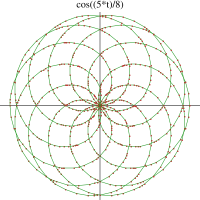
This is an example of FriCAS’s two-dimensional plotting. From the 2D Control Panel you can rescale the plot, turn axes and units on and off and save the image, among other things. This PostScript image was produced by clicking on the PS 2D Control Panel button.
draw(cos(5*t/8), t=0..16*%pi, coordinates==polar)
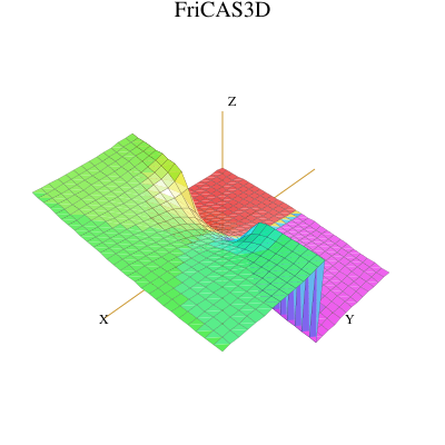
This is an example of FriCAS’s three-dimensional plotting. It is a monochrome graph of the complex arctangent function. The image displayed was rotated and had the “shade” and “outline” display options set from the 3D Control Panel. The PostScript output was produced by clicking on the save 3D Control Panel button and then clicking on the PS button. See Section 8.1 on page 479 for more details and examples of FriCAS’s numeric and graphics capabilities.
draw((x,y) +-> real atan complex(x,y), -%pi..%pi, -%pi..%pi, colorFunction == (x,y) +-> argument atan complex(x,y))
An exhibit of FriCAS Images is given in the center section of this book. For a description of the commands and programs that produced these figures, see Appendix A.27. PostScript output is available so that FriCAS images can be printed.4 See Chapter 7 for more examples and details about using FriCAS’s graphics facilities.
FriCAS distinguishes very carefully between different kinds of numbers, how they are represented and what their properties are. Here is a sampling of some of these kinds of numbers and some things you can do with them.
Integer arithmetic is always exact.
11^13 * 13^11 * 17^7 - 19^5 * 23^3
PositiveInteger Integers can be represented in factored form.
factor 643238070748569023720594412551704344145570763243
Factored(Integer) Results stay factored when you do arithmetic. Note that the 12 is automatically factored
for you.
% * 12
Factored(Integer) Integers can also be displayed to bases other than 10. This is an integer in base 11.
radix(25937424601,11)
RadixExpansion(11) Roman numerals are also available for those special occasions.
roman(1992)
RomanNumeral Rational number arithmetic is also exact.
r := 10 + 9/2 + 8/3 + 7/4 + 6/5 + 5/6 + 4/7 + 3/8 + 2/9
Fraction(Integer) To factor fractions, you have to map factor onto the numerator and denominator.
map(factor,r)
Fraction(Factored(Integer)) Type SingleInteger refers to machine word-length integers. In English, this expression
means “11 as a small integer”.
11@SingleInteger
SingleInteger Machine double-precision floating-point numbers are also available for numeric and graphical applications.
123.21@DoubleFloat
The normal floating-point type in FriCAS, Float, is a software implementation of floating-point numbers in which the exponent and the mantissa may have any number of digits.5 The types Complex(Float) and Complex(DoubleFloat) are the corresponding software implementations of complex floating-point numbers.
This is a floating-point approximation to about twenty digits. The “::” is used here to change from one kind of object (here, a rational number) to another (a floating-point number).
r :: Float
Float Use digits to change the number of digits in the representation. This operation returns the previous value so you can reset it later.
digits(22)
PositiveInteger To 22 digits of precision, the number  appears to be an integer.
exp(%pi * sqrt 163.0)
Float Increase the precision to forty digits and try again.
digits(40); exp(%pi * sqrt 163.0)
Float Here are complex numbers with rational numbers as real and imaginary parts.
(2/3 + %i)^3
Complex(Fraction(Integer)) The standard operations on complex numbers are available.
conjugate %
Complex(Fraction(Integer)) You can factor complex integers.
factor(89 - 23 * %i)
Factored(Complex(Integer)) Complex numbers with floating point parts are also available.
exp(%pi/4.0 * %i)
Complex(Float) Every rational number has an exact representation as a repeating decimal expansion (see ‘DecimalExpansion’ on page 813).
decimal(1/352)
DecimalExpansion A rational number can also be expressed as a continued fraction (see ‘ContinuedFraction’ on page 780).
continuedFraction(6543/210)
ContinuedFraction(Integer) Also, partial fractions can be used and can be displayed in a compact …
partialFraction(1,factorial(10))
PartialFraction(Integer) or expanded format (see ‘PartialFraction’ on page 1177).
padicFraction(%)
PartialFraction(Integer) Like integers, bases (radices) other than ten can be used for rational numbers (see ‘RadixExpansion’ on page 1208). Here we use base eight.
radix(4/7, 8)
RadixExpansion(8) Of course, there are complex versions of these as well. FriCAS decides to make the result a complex rational number.
% + 2/3*%i
Complex(Fraction(Integer)) You can also use FriCAS to manipulate fractional powers.
(5 + sqrt 63 + sqrt 847)^(1/3)
AlgebraicNumber You can also compute with integers modulo a prime.
x : PrimeField 7 := 5
PrimeField(7) Arithmetic is then done modulo  .
x^3
PrimeField(7) Since  is prime, you can invert nonzero values.
1/x
PrimeField(7) You can also compute modulo an integer that is not a prime.
y : IntegerMod 6 := 5
IntegerMod(6) All of the usual arithmetic operations are available.
y^3
IntegerMod(6) Inversion is not available if the modulus is not a prime number. Modular arithmetic and prime fields are discussed in Section 8.11.1 on page 599.
1/y
There are 10 exposed and 16 unexposed library operations named / having 2 argument(s) but none was determined to be applicable. Use HyperDoc Browse, or issue )display op / to learn more about the available operations. Perhaps package-calling the operation or using coercions on the arguments will allow you to apply the operation.
Cannot find a definition or applicable library operation named / with argument type(s) PositiveInteger IntegerMod(6) Perhaps you should use "@" to indicate the required return type, or "$" to specify which version of the function you need.
This defines a to be an algebraic number, that is, a root of a polynomial equation.
a := rootOf(a^5 + a^3 + a^2 + 3,a)
Expression(Integer) Computations with a are reduced according to the polynomial equation.
(a + 1)^10
Expression(Integer) Define b to be an algebraic number involving a.
b := rootOf(b^4 + a,b)
Expression(Integer) Do some arithmetic.
2/(b - 1)
Expression(Integer) To expand and simplify this, call ratDenom to rationalize the denominator.
ratDenom(%)
Expression(Integer) If we do this, we should get b.
2/%+1
Expression(Integer) But we need to rationalize the denominator again.
ratDenom(%)
Expression(Integer) Types Quaternion and Octonion are also available. Multiplication of quaternions is non-commutative, as expected.
q:=quatern(1,2,3,4)*quatern(5,6,7,8) - quatern(5,6,7,8)*quatern(1,2,3,4)
FriCAS has a large variety of data structures available. Many data structures are particularly useful for interactive computation and others are useful for building applications. The data structures of FriCAS are organized into category hierarchies as shown on the inside back cover.
A list is the most commonly used data structure in FriCAS for holding objects all of the same type.6 The name list is short for “linked-list of nodes.” Each node consists of a value (first) and a link (rest) that points to the next node, or to a distinguished value denoting the empty list. To get to, say, the third element, FriCAS starts at the front of the list, then traverses across two links to the third node.
Write a list of elements using square brackets with commas separating the elements.
u := [1,-7,11]
List(Integer) This is the value at the third node. Alternatively, you can say u.3.
first rest rest u
Many operations are defined on lists, such as: empty?, to test that a list has no elements; cons(x,l), to create
a new list with first element x and rest l; reverse, to create a new list with elements in reverse order; and sort,
to arrange elements in order.
An important point about lists is that they are “mutable”: their constituent elements and links can be changed “in place.” To do this, use any of the operations whose names end with the character “!”.
The operation concat!(u,v) replaces the last link of the list u to point to some other list v. Since u refers to
the original list, this change is seen by u.
concat!(u,[9,1,3,-4]); u
List(Integer) A cyclic list is a list with a “cycle”: a link pointing back to an earlier node of the list. To create a cycle, first get a node somewhere down the list.
lastnode := rest(u,3)
List(Integer) Use setrest! to change the link emanating from that node to point back to an earlier part of the list.
setrest!(lastnode,rest(u,2)); u
A stream is a structure that (potentially) has an infinite number of distinct elements.7 Think of a stream as an “infinite list” where elements are computed successively.
Create an infinite stream of factored integers. Only a certain number of initial elements are computed and displayed.
[factor(i) for i in 2.. by 2]
Stream(Factored(Integer)) FriCAS represents streams by a collection of already-computed elements together with a
function to compute the next element “on demand.” Asking for the  element causes elements
1 through n
to be evaluated.
%.36
Streams can also be finite or cyclic. They are implemented by a linked list structure similar to lists and have many of the same operations. For example, first and rest are used to access elements and successive nodes of a stream.
A one-dimensional array is another data structure used to hold objects of the same type.8 Unlike lists, one-dimensional arrays are inflexible—they are implemented using a fixed block of storage. Their advantage is that they give quick and constant access time to any element.
A simple way to create a one-dimensional array is to apply the operation oneDimensionalArray to a list of elements.
a := oneDimensionalArray [1, -7, 3, 3/2]
OneDimensionalArray(Fraction(Integer)) One-dimensional arrays are also mutable: you can change their constituent elements “in place.”
a.3 := 11; a
OneDimensionalArray(Fraction(Integer)) However, one-dimensional arrays are not flexible structures. You cannot destructively concat! them together.
concat!(a,oneDimensionalArray [1,-2])
There are 5 exposed and 0 unexposed library operations named concat! having 2 argument(s) but none was determined to be applicable. Use HyperDoc Browse, or issue )display op concat! to learn more about the available operations. Perhaps package-calling the operation or using coercions on the arguments will allow you to apply the operation.
Cannot find a definition or applicable library operation named concat! with argument type(s) OneDimensionalArray(Fraction(Integer)) OneDimensionalArray(Integer) Perhaps you should use "@" to indicate the required return type, or "$" to specify which version of the function you need.
Examples of datatypes similar to OneDimensionalArray are: Vector (vectors are mathematical structures implemented by one-dimensional arrays), String (arrays of “characters,” represented by byte vectors), and Bits (represented by “bit vectors”).
A vector of 32 bits, each representing the Boolean value true.
bits(32,true)
A flexible array is a cross between a list and a one-dimensional array.9 Like a one-dimensional array, a flexible array occupies a fixed block of storage. Its block of storage, however, has room to expand! When it gets full, it grows (a new, larger block of storage is allocated); when it has too much room, it contracts.
Create a flexible array of three elements.
f := flexibleArray [2, 7, -5]
FlexibleArray(Integer) Insert some elements between the second and third elements.
insert!(flexibleArray [11, -3],f,3)
Flexible arrays are used to implement “heaps.” A heap is an example of a data structure called a priority queue, where elements are ordered with respect to one another.10 A heap is organized so as to optimize insertion and extraction of maximum elements. The extract! operation returns the maximum element of the heap, after destructively removing that element and reorganizing the heap so that the next maximum element is ready to be delivered.
An easy way to create a heap is to apply the operation heap to a list of values.
h := heap [-4,7,11,3,4,-7]
Heap(Integer) This loop extracts elements one-at-a-time from h until the heap is exhausted, returning the
elements as a list in the order they were extracted.
[extract!(h) while not empty?(h)]
A binary tree is a “tree” with at most two branches per node: it is either empty, or else is a node consisting of a value, and a left and right subtree (again, binary trees).11
A binary search tree is a binary tree such that, for each node, the value of the node is greater than all values (if any) in the left subtree, and less than or equal to all values (if any) in the right subtree.
binarySearchTree [5,3,2,9,4,7,11]
BinarySearchTree(PositiveInteger)
A balanced binary tree is useful for doing modular computations. Given a list lm of moduli, modTree(a,lm)
produces a balanced binary tree with the values  at its leaves.
modTree(8,[2,3,5,7])
A set is a collection of elements where duplication and order is irrelevant.12 Sets are always finite and have no corresponding structure like streams for infinite collections.
Create sets by using the set function.
fs := set[1/3,4/5,-1/3,4/5]
A multiset is a set that keeps track of the number of duplicate
values.13
For all the primes p between 2 and 1000, find the distribution of  .
multiset [x rem 5 for x in primes(2,1000)]
A table is conceptually a set of “key–value” pairs and is a generalization of a multiset.14 The domain Table(Key, Entry) provides a general-purpose type for tables with values of type Entry indexed by keys of type Key.
Compute the above distribution of primes using tables. First, let t denote an empty table of keys and values,
each of type Integer.
t : Table(Integer,Integer) := empty()
We define a function howMany to return the number of values of a given modulus k seen so far. It calls
search(k,t) which returns the number of values stored under the key k in table t, or "failed" if no such
value is yet stored in t under k.
In English, this says “Define howMany(k) as follows. First, let  be the value of search
 . Then, if
 has
the value
 , return the value
 ; otherwise return
 .”
howMany(k) == (n:=search(k,t); n case "failed" => 1; n+1)
Run through the primes to create the table, then print the table. The expression t.m := howMany(m) updates
the value in table t stored under key m.
for p in primes(2,1000) repeat (m:= p rem 5; t.m:= howMany(m)); t
Compiling function howMany with type Integer -> Integer
A record is an example of an inhomogeneous collection of objects.15 A record consists of a set of named selectors that can be used to access its components.
Declare that daniel can only be assigned a record with two prescribed fields.
daniel : Record(age : Integer, salary : Float)
Give daniel a value, using square brackets to enclose the values of the fields.
daniel := [28, 32005.12]
Record(age: Integer, salary: Float) Give daniel a raise.
daniel.salary := 35000; daniel
Record(age: Integer, salary: Float)
A union is a data structure used when objects have multiple types.16
Let dog be either an integer or a string value.
dog: Union(licenseNumber: Integer, name: String)
Give dog a name.
dog := "Whisper"
All told, there are over forty different data structures in FriCAS. Using the domain constructors described in Chapter 13, you can add your own data structure or extend an existing one. Choosing the right data structure for your application may be the key to obtaining good performance.
To get higher dimensional aggregates, you can create one-dimensional aggregates with elements that are themselves aggregates, for example, lists of lists, one-dimensional arrays of lists of multisets, and so on. For applications requiring two-dimensional homogeneous aggregates, you will likely find two-dimensional arrays and matrices most useful.
The entries in TwoDimensionalArray and Matrix objects are all the same type, except that those for Matrix must belong to a Ring. You create and access elements in roughly the same way. Since matrices have an understood algebraic structure, certain algebraic operations are available for matrices but not for arrays. Because of this, we limit our discussion here to Matrix, that can be regarded as an extension of TwoDimensionalArray.17
You can create a matrix from a list of lists, where each of the inner lists represents a row of the matrix.
m := matrix([[1,2], [3,4]])
Matrix(Integer) The “collections” construct (see Section 5.5 on page 283) is useful for creating matrices whose entries are given by formulas.
matrix([[1/(i + j - x) for i in 1..4] for j in 1..4])
Matrix(Fraction(Polynomial(Integer))) Let vm denote the three by three Vandermonde matrix.
vm := matrix [[1,1,1], [x,y,z], [x*x,y*y,z*z]]
Matrix(Polynomial(Integer)) Use this syntax to extract an entry in the matrix.
vm(3,3)
Polynomial(Integer) You can also pull out a row or a column.
column(vm,2)
Vector(Polynomial(Integer)) You can do arithmetic.
vm * vm
Matrix(Polynomial(Integer)) You can perform operations such as transpose, trace, and determinant.
factor determinant vm
FriCAS provides you with a very large library of predefined operations and objects to compute with. You can use the FriCAS library of constructors to create new objects dynamically of quite arbitrary complexity. For example, you can make lists of matrices of fractions of polynomials with complex floating point numbers as coefficients. Moreover, the library provides a wealth of operations that allow you to create and manipulate these objects.
For many applications, you need to interact with the interpreter and write some FriCAS programs to tackle your application. FriCAS allows you to write functions interactively, thereby effectively extending the system library. Here we give a few simple examples, leaving the details to Chapter 6.
We begin by looking at several ways that you can define the “factorial” function in FriCAS. The first way is to give a piece-wise definition of the function. This method is best for a general recurrence relation since the pieces are gathered together and compiled into an efficient iterative function. Furthermore, enough previously computed values are automatically saved so that a subsequent call to the function can pick up from where it left off.
Define the value of fact at 0.
fact(0) == 1
Define the value of fact(n) for general n.
fact(n) == n*fact(n-1)
Ask for the value at 50. The resulting function created by FriCAS computes the value by iteration.
fact(50)
Compiling function fact with type Integer -> Integer
Compiling function fact as a recurrence relation.
PositiveInteger A second definition uses an if-then-else and recursion.
fac(n) == if n < 3 then n else n * fac(n - 1)
This function is less efficient than the previous version since each iteration involves a recursive function call.
fac(50)
Compiling function fac with type Integer -> Integer
PositiveInteger A third version directly uses iteration.
fa(n) == (a := 1; for i in 2..n repeat a := a*i; a)
This is the least space-consuming version.
fa(50)
Compiling function fa with type PositiveInteger -> PositiveInteger
PositiveInteger A final version appears to construct a large list and then reduces over it with multiplication.
f(n) == reduce(*,[i for i in 2..n])
In fact, the resulting computation is optimized into an efficient iteration loop equivalent to that of the third version.
f(50)
Compiling function f with type PositiveInteger -> PositiveInteger
PositiveInteger The library version uses an algorithm that is different from the four above because it highly optimizes the recurrence relation definition of factorial.
factorial(50)
You are not limited to one-line functions in FriCAS. If you place your function definitions in .input files (see Section 4.1 on page 207), you can have multi-line functions that use indentation for grouping.
Given n elements, diagonalMatrix creates an n by n matrix with those elements down the diagonal. This
function uses a permutation matrix that interchanges the ith and jth rows of a matrix by which it is
right-multiplied.
This function definition shows a style of definition that can be used in .input files. Indentation is used to
create blocks: sequences of expressions that are evaluated in sequence except as modified by control statements
such as if-then-else and return.
permMat(n, i, j) == m := diagonalMatrix [(if i = k or j = k then 0 else 1) for k in 1..n] m(i,j) := 1 m(j,i) := 1 m
This creates a four by four matrix that interchanges the second and third rows.
p := permMat(4,2,3)
Compiling function permMat with type (PositiveInteger, PositiveInteger, PositiveInteger) -> Matrix(NonNegativeInteger)
Matrix(NonNegativeInteger) Create an example matrix to permute.
m := matrix [[4*i + j for j in 1..4] for i in 0..3]
Matrix(NonNegativeInteger) Interchange the second and third rows of m.
permMat(4,2,3) * m
A function can also be passed as an argument to another function, which then applies the function or passes it off to some other function that does. You often have to declare the type of a function that has functional arguments.
This declares t to be a two-argument function that returns a Float. The first argument is a function that takes one Float argument and returns a Float.
t : (Float -> Float, Float) -> Float
t(fun, x) == fun(x)^2 + sin(x)^2
We have not defined a cos in the workspace. The one from the FriCAS library will do.
t(cos, 5.2058)
Compiling function t with type ((Float -> Float), Float) -> Float
Float Here we define our own (user-defined) function.
cosinv(y) == cos(1/y)
Pass this function as an argument to t.
t(cosinv, 5.2058)
Compiling function cosinv with type Float -> Float
FriCAS also has pattern matching capabilities for simplification of expressions and for defining new functions by rules. For example, suppose that you want to apply regularly a transformation that groups together products of radicals:

Note that such a transformation is not generally correct. FriCAS never uses it automatically.
Give this rule the name groupSqrt.
groupSqrt := rule(sqrt(a) * sqrt(b) == sqrt(a*b))
RewriteRule(Integer, Integer, Expression(Integer)) Here is a test expression.
a := (sqrt(x) + sqrt(y) + sqrt(z))^4
Expression(Integer) The rule groupSqrt successfully simplifies the expression.
groupSqrt a
Polynomials are the commonly used algebraic types in symbolic computation. Interactive users
of FriCAS generally only see one type of polynomial: Polynomial(R). This type represents
polynomials in any number of unspecified variables over a particular coefficient domain R. This
type represents its coefficients sparsely: only terms with non-zero coefficients are represented.
In building applications, many other kinds of polynomial representations are useful. Polynomials may have one variable or multiple variables, the variables can be named or unnamed, the coefficients can be stored sparsely or densely. So-called “distributed multivariate polynomials” store polynomials as coefficients paired with vectors of exponents. This type is particularly efficient for use in algorithms for solving systems of non-linear polynomial equations.
The polynomial constructor most familiar to the interactive user is Polynomial.
(x^2 - x*y^3 +3*y)^2
Polynomial(Integer) If you wish to restrict the variables used, UnivariatePolynomial provides polynomials in one variable.
p: UP(x,INT) := (3*x-1)^2 * (2*x + 8)
UnivariatePolynomial(x, Integer) The constructor MultivariatePolynomial provides polynomials in one or more specified variables.
m: MPOLY([x,y],INT) := (x^2-x*y^3+3*y)^2
MultivariatePolynomial([x, y], Integer) You can change the way the polynomial appears by modifying the variable ordering in the explicit list.
m :: MPOLY([y,x],INT)
MultivariatePolynomial([y, x], Integer) The constructor DistributedMultivariatePolynomial provides polynomials in one or more specified variables with the monomials ordered lexicographically.
m :: DMP([y,x],INT)
DistributedMultivariatePolynomial([y, x], Integer) The constructor HomogeneousDistributedMultivariatePolynomial is similar except that the monomials are ordered by total order refined by reverse lexicographic order.
m :: HDMP([y,x],INT)
HomogeneousDistributedMultivariatePolynomial([y, x], Integer)
More generally, the domain constructor GeneralDistributedMultivariatePolynomial allows the user to provide an arbitrary predicate to define their own term ordering. These last three constructors are typically used in Gröbner basis applications and when a flat (that is, non-recursive) display is wanted and the term ordering is critical for controlling the computation.
FriCAS’s limit function is usually used to evaluate limits of quotients where the numerator and denominator
both tend to zero or both tend to infinity. To find the limit of an expression f as a real variable x tends to a
limit value a, enter limit(f, x=a). Use complexLimit if the variable is complex. Additional information and
examples of limits are in Section 8.6 on page 533.
You can take limits of functions with parameters.
g := csc(a*x) / csch(b*x)
Expression(Integer) As you can see, the limit is expressed in terms of the parameters.
limit(g,x=0)
Union(OrderedCompletion(Expression(Integer)), ...) A variable may also approach plus or minus infinity:
h := (1 + k/x)^x
Expression(Integer) Use %plusInfinity and %minusInfinity to denote  and
 .
limit(h,x=%plusInfinity)
Union(OrderedCompletion(Expression(Integer)), ...) A function can be defined on both sides of a particular value, but may tend to different limits as its variable approaches that value from the left and from the right.
limit(sqrt(y^2)/y,y = 0)
Union(Record(leftHandLimit: Union(OrderedCompletion(Expression(Integer)), "failed"), rightHandLimit: Union(OrderedCompletion(Expression(Integer)), "failed")), ...) As x approaches 0 along the real axis, exp(-1/x^2) tends to 0.
limit(exp(-1/x^2),x = 0)
Union(OrderedCompletion(Expression(Integer)), ...) However, if x is allowed to approach 0 along any path in the complex plane, the limiting
value of exp(-1/x^2) depends on the path taken because the function has an essential singularity at x=0.
This is reflected in the error message returned by the function.
complexLimit(exp(-1/x^2),x = 0)
FriCAS also provides power series. By default, FriCAS tries to compute and display the first ten elements of a series. Use )set streams calculate to change the default value to something else. For the purposes of this book, we have used this system command to display fewer than ten terms. For more information about working with series, see Section 8.9 on page 549.
You can convert a functional expression to a power series by using the operation series. In this example,
sin(a*x) is expanded in powers of (x - 0), that is, in powers of x.
series(sin(a*x),x = 0)
UnivariatePuiseuxSeries(Expression(Integer), x, 0) This expression expands sin(a*x) in powers of (x - %pi/4).
series(sin(a*x),x = %pi/4)
UnivariatePuiseuxSeries(Expression(Integer), x, \%pi/4) FriCAS provides Puiseux series: series with rational number exponents.
The first argument to series is an in-place function that computes the  coefficient. (Recall that the “+->”
is an infix operator meaning “maps to.”)
series(n +-> (-1)^((3*n - 4)/6)/factorial(n - 1/3),x = 0,4/3..,2)
UnivariatePuiseuxSeries(Expression(Integer), x, 0) Once you have created a power series, you can perform arithmetic
operations on that series. We compute the Taylor expansion of 1/(1-x).
f := series(1/(1-x),x = 0)
UnivariatePuiseuxSeries(Expression(Integer), x, 0) Compute the square of the series.
f ^ 2
UnivariatePuiseuxSeries(Expression(Integer), x, 0) The usual elementary functions (log, exp, trigonometric functions, and so on) are defined for power series.
f := series(1/(1-x),x = 0)
UnivariatePuiseuxSeries(Expression(Integer), x, 0)
g := log(f)
UnivariatePuiseuxSeries(Expression(Integer), x, 0)
exp(g)
UnivariatePuiseuxSeries(Expression(Integer), x, 0) Here is a way to obtain numerical approximations of e from the Taylor
series expansion of exp(x). First create the desired Taylor expansion.
f := taylor(exp(x))
UnivariateTaylorSeries(Expression(Integer), x, 0) Evaluate the series at the value 1.0. As you see, you get a sequence of
partial sums.
eval(f,1.0)
Use the FriCAS function D to differentiate an expression.
To find the derivative of an expression f with respect to a variable x, enter D(f, x).
f := exp exp x
D(f, x)
Expression(Integer) An optional third argument n in D asks FriCAS for the  derivative of
f. This finds
the fourth derivative of f with respect to x.
D(f, x, 4)
Expression(Integer) You can also compute partial derivatives by specifying the order of differentiation.
g := sin(x^2 + y)
D(g, y)
D(g, [y, y, x, x])
FriCAS can manipulate the derivatives (partial and iterated) of expressions involving formal operators. All the
dependencies must be explicit. This returns 0 since F (so far) does not explicitly depend on
x.
D(F,x)
Polynomial(Integer) Suppose that we have F a function of x, y, and z, where x and y are themselves functions
of z. Start by declaring that F, x, and y are operators.
F := operator ’F; x := operator ’x; y := operator ’y
BasicOperator You can use F, x, and y in expressions.
a := F(x z, y z, z^2) + x y(z+1)
Expression(Integer) Differentiate formally with respect to z. The formal derivatives appearing in dadz are
not just formal symbols, but do represent the derivatives of x, y, and F.
dadz := D(a, z)
Expression(Integer) You can evaluate the above for particular functional values of F, x, and y. If x(z) is
exp(z) and y(z) is log(z+1), then this evaluates dadz.
eval(eval(dadz, ’x, z +-> exp z), ’y, z +-> log(z+1))
Expression(Integer) You obtain the same result by first evaluating a and then differentiating.
eval(eval(a, ’x, z +-> exp z), ’y, z +-> log(z+1))
D(%, z)
FriCAS has extensive library facilities for integration.
The first example is the integration of a fraction with denominator that factors into a quadratic and a quartic irreducible polynomial. The usual partial fraction approach used by most other computer algebra systems either fails or introduces expensive unneeded algebraic numbers.
We use a factorization-free algorithm.
integrate((x^2+2*x+1)/((x+1)^6+1),x)
Union(Expression(Integer), ...)
When real parameters are present, the form of the integral can depend on the signs of some expressions.
Rather than query the user or make sign assumptions, FriCAS returns all possible answers.
integrate(1/(x^2 + a),x)
Union(List(Expression(Integer)), ...)
The integrate operation generally assumes that all parameters are real. The only exception is when the integrand has complex valued quantities.
If the parameter is complex instead of real, then the notion of sign is undefined and there is a unique answer. You can request this answer by “prepending” the word “complex” to the command name:
complexIntegrate(1/(x^2 + a),x)
The following two examples illustrate the limitations of table-based approaches. The two integrands are very similar, but the answer to one of them requires the addition of two new algebraic numbers.
This one is the easy one. The next one looks very similar but the answer is much more complicated.
integrate(x^3 / (a+b*x)^(1/3),x)
Union(Expression(Integer), ...) Only an algorithmic approach is guaranteed to find what new constants must be added in order to find a solution.
integrate(1 / (x^3 * (a+b*x)^(1/3)),x)
Union(Expression(Integer), ...)
Some computer algebra systems use heuristics or table-driven approaches to integration. When these systems cannot determine the answer to an integration problem, they reply “I don’t know.” FriCAS uses an algorithm for integration that conclusively proves that an integral cannot be expressed in terms of elementary functions.
When FriCAS returns an integral sign, it has proved that no answer exists as an elementary function.
integrate(log(1 + sqrt(a*x + b)) / x,x)
Union(Expression(Integer), ...) FriCAS can handle complicated mixed functions much beyond what you can find in tables. Whenever possible, FriCAS tries to express the answer using the functions present in the integrand.
integrate((sinh(1+sqrt(x+b))+2*sqrt(x+b)) / (sqrt(x+b) * (x + cosh(1+sqrt(x + b)))), x)
Union(Expression(Integer), ...) A strong structure-checking algorithm in FriCAS finds hidden algebraic relationships between functions.
integrate(tan(atan(x)/3),x)
Union(Expression(Integer), ...) The discovery of this algebraic relationship is necessary for correct integration of this function. Here are the details:
If  and
 then the following algebraic relation is true:

Integrate g using this algebraic relation; this produces:

Rationalize the denominator, producing:

Replace g by the initial definition  to produce the final result.
This is an example of a mixed function where the algebraic layer is over the transcendental one.
integrate((x + 1) / (x*(x + log x) ^ (3/2)), x)
Union(Expression(Integer), ...) While incomplete for non-elementary functions, FriCAS can handle some of them.
integrate(exp(-x^2) * erf(x) / (erf(x)^3 - erf(x)^2 - erf(x) + 1),x)
Union(Expression(Integer), ...)
More examples of FriCAS’s integration capabilities are discussed in Section 8.8 on page 543.
The general approach used in integration also carries over to the solution of linear differential equations.
Let’s solve some differential equations. Let y be the unknown function in terms of x.
y := operator ’y
BasicOperator Here we solve a third order equation with polynomial coefficients.
deq := x^3 * D(y x, x, 3) + x^2 * D(y x, x, 2) - 2 * x * D(y x, x) + 2 * y x = 2 * x^4
solve(deq, y, x)
Union(Record(particular: Expression(Integer), basis: List(Expression(Integer))), ...) Here we find all the algebraic function solutions of the equation.
deq := (x^2 + 1) * D(y x, x, 2) + 3 * x * D(y x, x) + y x = 0
solve(deq, y, x)
Union(Record(particular: Expression(Integer), basis: List(Expression(Integer))), ...)
Coefficients of differential equations can come from arbitrary constant fields. For example, coefficients can contain algebraic numbers.
This example has solutions whose logarithmic derivative is an algebraic function of degree two.
eq := 2*x^3 * D(y x,x,2) + 3*x^2 * D(y x,x) - 2 * y x
solve(eq,y,x).basis
Here’s another differential equation to solve.
deq := D(y x, x) = y(x) / (x + y(x) * log y x)
solve(deq, y, x)
Union(Expression(Integer), ...)
Rather than attempting to get a closed form solution of a differential equation, you instead might want to find an approximate solution in the form of a series.
Let’s solve a system of nonlinear first order equations and get a solution in power series. Tell FriCAS that x is
also an operator.
x := operator ’x
BasicOperator Here are the two equations forming our system.
eq1 := D(x(t), t) = 1 + x(t)^2
eq2 := D(y(t), t) = x(t) * y(t)
Equation(Expression(Integer)) We can solve the system around t = 0 with the initial conditions x(0)= 0 and y(0)= 1.
Notice that since we give the unknowns in the order [x, y], the answer is a list of two series in the order
[series for x(t), series for y(t)].
seriesSolve([eq2, eq1], [x, y], t = 0, [y(0) = 1, x(0) = 0])
Compiling function %JL with type List(UnivariateTaylorSeries(Expression(Integer ),t,0)) -> UnivariateTaylorSeries(Expression(Integer),t,0)
Compiling function %JM with type List(UnivariateTaylorSeries(Expression(Integer ),t,0)) -> UnivariateTaylorSeries(Expression(Integer),t,0)
List(UnivariateTaylorSeries(Expression(Integer), t, 0))
FriCAS also has state-of-the-art algorithms for the solution of systems of polynomial equations. When the number of equations and unknowns is the same, and you have no symbolic coefficients, you can use solve for real roots and complexSolve for complex roots. In each case, you tell FriCAS how accurate you want your result to be. All operations in the solve family return answers in the form of a list of solution sets, where each solution set is a list of equations.
A system of two equations involving a symbolic parameter t.
S(t) == [x^2-2*y^2 - t,x*y-y-5*x + 5]
Find the real roots of S(19) with rational arithmetic, correct to within  .
solve(S(19),1/10^20)
Compiling function S with type PositiveInteger -> List(Polynomial(Integer))
List(List(Equation(Polynomial(Fraction(Integer))))) Find the complex roots of S(19) with floating point coefficients to 20 digits accuracy in the
mantissa.
complexSolve(S(19),10.e-20)
List(List(Equation(Polynomial(Complex(Float))))) If a system of equations has symbolic coefficients and you want a solution in radicals, try radicalSolve.
radicalSolve(S(a),[x,y])
Compiling function S with type Variable(a) -> List(Polynomial(Integer))
List(List(Equation(Expression(Integer)))) For systems of equations with symbolic coefficients, you can apply solve, listing the variables that you want FriCAS to solve for. For polynomial equations, a solution cannot usually be expressed solely in terms of the other variables. Instead, the solution is presented as a “triangular” system of equations, where each polynomial has coefficients involving only the succeeding variables. This is analogous to converting a linear system of equations to “triangular form”. A system of three equations in five variables.
eqns := [x^2 - y + z,x^2*z + x^4 - b*y, y^2 *z - a - b*x]
List(Polynomial(Integer)) Solve the system for unknowns  , reducing the solution to triangular
form.
solve(eqns,[x,y,z])
List(List(Equation(Fraction(Polynomial(Integer)))))
We conclude our tour of FriCAS with a brief discussion of system commands. System commands are special statements that start with a closing parenthesis (“)”). They are used to control or display your FriCAS environment, start the HyperDoc system, issue operating system commands and leave FriCAS. For example, )system is used to issue commands to the operating system from FriCAS. Here is a brief description of some of these commands. For more information on specific commands, see Appendix 15.4.10.
Perhaps the most important user command is the )clear all command that initializes your environment.
Every section and subsection in this book has an invisible )clear all that is read prior to the examples
given in the section. )clear all gives you a fresh, empty environment with no user variables defined and the
step number reset to 1. The )clear command can also be used to selectively clear values and properties of
system variables.
Another useful system command is )read. A preferred way to develop an application in FriCAS is to put your interactive commands into a file, say my.input file. To get FriCAS to read this file, you use the system command )read my.input. If you need to make changes to your approach or definitions, go into your favorite editor, change my.input, then )read my.input again.
Other system commands include: )history, to display previous input and/or output lines; )display, to display properties and values of workspace variables; and )what.
Issue )what to get a list of FriCAS objects that contain a given substring in their name.
)what operations integrate
Operations whose names satisfy the above pattern(s): HermiteIntegrate algintegrate complexIntegrate expintegrate fintegrate infieldIntegrate integrate integrateIfCan integrate_sols internalIntegrate internalIntegrate0 lambintegrate lazyGintegrate lazyIntegrate lfintegrate monomialIntegrate palgintegrate pmintegrate primintegrate To get more information about an operation such as integrate , issue the command )display op integrate
A useful system command is )undo. Sometimes while computing interactively with FriCAS, you make a mistake and enter an incorrect definition or assignment. Or perhaps you need to try one of several alternative approaches, one after another, to find the best way to approach an application. For this, you will find the undo facility of FriCAS helpful.
System command )undo n means “undo back to step n”; it restores the values of user variables to those that
existed immediately after input expression n was evaluated. Similarly, )undo -n undoes changes caused by the
last n input expressions. Once you have done an )undo, you can continue on from there, or make a change and
redo all your input expressions from the point of the )undo forward. The )undo is completely
general: it changes the environment like any user expression. Thus you can )undo any previous
undo.
Here is a sample dialogue between user and FriCAS. “Let me define two mutually dependent functions f and
g piece-wise.”
f(0) == 1; g(0) == 1
“Here is the general term for f.”
f(n) == e/2*f(n-1) - x*g(n-1)
“And here is the general term for g.”
g(n) == -x*f(n-1) + d/3*g(n-1)
“What is the value of f(3)?”
f(3)
Compiling function g with type Integer -> Polynomial(Fraction(Integer))
Compiling function g as a recurrence relation.
Compiling function g with type Integer -> Polynomial(Fraction(Integer))
Compiling function g as a recurrence relation.
Compiling function f with type Integer -> Polynomial(Fraction(Integer))
Compiling function f as a recurrence relation.
Polynomial(Fraction(Integer)) “Hmm, I think I want to define f differently. Undo to the environment right after I
defined f.”
)undo 2
“Here is how I think I want f to be defined instead.”
f(n) == d/3*f(n-1) - x*g(n-1)
1 old definition(s) deleted for function or rule f
Redo the computation from expression 3 forward.
)undo )redo
“I want my old definition of f after all. Undo the undo and restore the environment to that immediately after
(4).”
)undo 4
“Check that the value of f(3) is restored.”
f(3)
Compiling function g with type Integer -> Polynomial(Fraction(Integer))
Compiling function g as a recurrence relation.
Compiling function g with type Integer -> Polynomial(Fraction(Integer))
Compiling function g as a recurrence relation.
Compiling function f with type Integer -> Polynomial(Fraction(Integer))
Compiling function f as a recurrence relation.
After you have gone off on several tangents, then backtracked to previous points in your conversation using )undo, you might want to save all the “correct” input commands you issued, disregarding those undone. The system command )history )write mynew.input writes a clean straight-line program onto the file mynew.input on your disk.
This concludes your tour of FriCAS. To disembark, issue the system command )quit to leave FriCAS and return to the operating system.
In this chapter we look at the key notion of type and its generalization mode. We show that every FriCAS object has a type that determines what you can do with the object. In particular, we explain how to use types to call specific functions from particular parts of the library and how types and modes can be used to create new objects from old. We also look at Record and Union types and the special type Any. Finally, we give you an idea of how FriCAS manipulates types and modes internally to resolve ambiguities.
The FriCAS world deals with many kinds of objects. There are mathematical objects such as numbers and polynomials, data structure objects such as lists and arrays, and graphics objects such as points and graphic images. Functions are objects too.
FriCAS organizes objects using the notion of domain of computation, or simply domain. Each domain denotes a class of objects. The class of objects it denotes is usually given by the name of the domain: Integer for the integers, Float for floating-point numbers, and so on. The convention is that the first letter of a domain name is capitalized. Similarly, the domain Polynomial(Integer) denotes “polynomials with integer coefficients.” Also, Matrix(Float) denotes “matrices with floating-point entries.”
Every basic FriCAS object belongs to a unique domain. The integer 3 belongs to the domain Integer and the
polynomial x + 3 belongs to the domain Polynomial(Integer). The domain of an object is also called its type.
Thus we speak of “the type Integer” and “the type Polynomial(Integer).”
After an FriCAS computation, the type is displayed toward the right-hand side of the page (or screen).
-3
Integer Here we create a rational number but it looks like the last result. The type, however, tells you it is different. You cannot identify the type of an object by how FriCAS displays the object.
-3/1
Fraction(Integer) When a computation produces a result of a simpler type, FriCAS leaves the type unsimplified. Thus no information is lost.
x + 3 - x
Polynomial(Integer) This seldom matters since FriCAS retracts the answer to the simpler type if it is necessary.
factorial(%)
Expression(Integer) When you issue a positive number, the type PositiveInteger is printed. Surely, 3 also
has type Integer! The curious reader may now have two questions. First, is the type of an object not unique?
Second, how is PositiveInteger related to Integer? Read on!
3
Any domain can be refined to a subdomain by a membership
predicate.1
For example, the domain Integer can be refined to the subdomain PositiveInteger, the set of
integers x such that x > 0, by giving the FriCAS predicate x . Similarly, FriCAS can define
subdomains such as “the subdomain of diagonal matrices,” “the subdomain of lists of length two,” “the
subdomain of monic irreducible polynomials in  x > 0
x,” and so on. Trivially, any domain is a subdomain of
itself.
While an object belongs to a unique domain, it can belong to any number of subdomains. Any subdomain of
the domain of an object can be used as the type of that object. The type of 3 is indeed both
Integer and PositiveInteger as well as any other subdomain of Integer whose predicate is
satisfied, such as “the prime integers,” “the odd positive integers between 3 and 17,” and so
on.
In FriCAS, domains are objects. You can create them, pass them to functions, and, as we’ll see later, test them for certain properties.
In FriCAS, you ask for a value of a function by applying its name to a set of arguments.
To ask for “the factorial of 7” you enter this expression to FriCAS. This applies the function factorial to the
value 7 to compute the result.
factorial(7)
PositiveInteger Enter the type Polynomial (Integer) as an expression to FriCAS. This looks much like a function call as well. It is! The result is stated to be of type Type, which according to our usual convention, denotes the class of all domains.
Polynomial(Integer)
The most basic operation involving domains is that of building a new domain from a given one. To create the domain of “polynomials over the integers,” FriCAS applies the function Polynomial to the domain Integer. A function like Polynomial is called a domain constructor or, more simply, a constructor. A domain constructor is a function that creates a domain. An argument to a domain constructor can be another domain or, in general, an arbitrary kind of object. Polynomial takes a single domain argument while SquareMatrix takes a positive integer as an argument to give its dimension and a domain argument to give the type of its components.
What kinds of domains can you use as the argument to Polynomial or SquareMatrix or List? Well, the first two are mathematical in nature. You want to be able to perform algebraic operations like + and * on polynomials and square matrices, and operations such as determinant on square matrices. So you want to allow polynomials of integers and polynomials of square matrices with complex number coefficients and, in general, anything that “makes sense.” At the same time, you don’t want FriCAS to be able to build nonsense domains such as “polynomials of strings!”
In contrast to algebraic structures, data structures can hold any kind of object. Operations on lists such as insert, delete, and concat just manipulate the list itself without changing or operating on its elements. Thus you can build List over almost any datatype, including itself. Create a complicated algebraic domain.
List (List (Matrix (Polynomial (Complex (Fraction (Integer))))))
Type Try to create a meaningless domain.
Polynomial(String)
Polynomial(String) is not a valid type.
Evidently from our last example, FriCAS has some mechanism that tells what a constructor can use as an argument. This brings us to the notion of category. As domains are objects, they too have a domain. The domain of a domain is a category. A category is simply a type whose members are domains.
A common algebraic category is Ring, the class of all domains that are “rings.” A ring is an algebraic
structure with constants 0 and 1 and operations +, -, and *. These operations are assumed “closed” with
respect to the domain, meaning that they take two objects of the domain and produce a result object also in
the domain. The operations are understood to satisfy certain “axioms,” certain mathematical principles
providing the algebraic foundation for rings. For example, the additive inverse axiom for rings states:
Every element x has an additive inverse y such that x + y = 0.
The prototypical example of a domain that is a ring is the integers. Keep them in mind whenever we mention Ring.
Many algebraic domain constructors such as Complex, Polynomial, Fraction, take rings as arguments and
return rings as values. You can use the infix operator “has” to ask a domain if it belongs to a particular
category.
All numerical types are rings. Domain constructor Polynomial builds “the ring of polynomials over any other ring.”
Polynomial(Integer) has Ring
Boolean Constructor List never produces a ring.
List(Integer) has Ring
Boolean The constructor Matrix(R) builds “the domain of all matrices over the ring R.” This
domain is never a ring since the operations “+”, “-”, and “*” on matrices of arbitrary shapes are
undefined.
Matrix(Integer) has Ring
Boolean Thus you can never build polynomials over matrices.
Polynomial(Matrix(Integer))
Polynomial(Matrix(Integer)) is not a valid type.
Use SquareMatrix(n,R) instead. For any positive integer n, it builds “the ring of n by n matrices over
R.”
Polynomial(SquareMatrix(7,Complex(Integer)))
Another common category is Field, the class of all fields. A field is a ring with additional
operations. For example, a field has commutative multiplication and a closed operation / for
the division of two elements. Integer is not a field since, for example, 3/2 does not have an
integer result. The prototypical example of a field is the rational numbers, that is, the domain
Fraction(Integer). In general, the constructor Fraction takes a ring as an argument and returns a
field.2
Other domain constructors, such as Complex, build fields only if their argument domain is a
field.
The complex integers (often called the “Gaussian integers”) do not form a field.
Complex(Integer) has Field
Boolean But fractions of complex integers do.
Fraction(Complex(Integer)) has Field
Boolean The algebraically equivalent domain of complex rational numbers is a field since domain constructor Complex produces a field whenever its argument is a field.
Complex(Fraction(Integer)) has Field
The most basic category is Type. It denotes the class of all domains and
subdomains.3
Domain constructor List is able to build “lists of elements from domain D” for arbitrary D simply by requiring
that D belong to category Type.
Now, you may ask, what exactly is a category? Like domains, categories can be defined in the FriCAS language. A category is defined by three components:
This last component is a new idea. And it is key to the design of FriCAS! Because categories can extend one another, they form hierarchies. Detailed charts showing the category hierarchies in FriCAS are displayed in the endpages of this book. There you see that all categories are extensions of Type and that Field is an extension of Ring.
The operations supported by the domains of a category are called the exports of that category because these are the operations made available for system-wide use. The exports of a domain of a given category are not only the ones explicitly mentioned by the category. Since a category extends other categories, the operations of these other categories—and all categories these other categories extend—are also exported by the domains.
For example, polynomial domains belong to PolynomialCategory. This category explicitly mentions some twenty-nine operations on polynomials, but it extends eleven other categories (including Ring). As a result, the current system has over one hundred operations on polynomials.
If a domain belongs to a category that extends, say, Ring, it is convenient to say that the domain exports Ring. The name of the category thus provides a convenient shorthand for the list of operations exported by the category. Rather than listing operations such as + and * of Ring each time they are needed, the definition of a type simply asserts that it exports category Ring.
The category name, however, is more than a shorthand. The name Ring, in fact, implies that the operations exported by rings are required to satisfy a set of “axioms” associated with the name Ring.4
Why is it not correct to assume that some type is a ring if it exports all of the operations of
Ring? Here is why. Some languages such as APL denote the Boolean constants true and false
by the integers 1 and 0 respectively, then use + and * to denote the logical operators or and
and. But with these definitions Boolean is not a ring since the additive inverse axiom is
violated.5
This alternative definition of Boolean can be easily and correctly implemented in FriCAS, since Boolean
simply does not assert that it is of category Ring. This prevents the system from building meaningless
domains such as Polynomial(Boolean) and then wrongfully applying algorithms that presume that the ring
axioms hold.
Enough on categories. To learn more about them, see Chapter 12. We now return to our discussion of domains.
Domains export a set of operations to make them available for system-wide use. Integer, for example,
exports the operations + and = given by the signatures +: (Integer,Integer) and =:
 Integer
(Integer,Integer), respectively. Each of these operations takes two Integer arguments. The +
operation also returns an Integer but = returns a Boolean:  Boolean
true or false. The operations exported by a
domain usually manipulate objects of the domain—but not always.
The operations of a domain may actually take as arguments, and return as values, objects from any domain.
For example, Fraction (Integer) exports the operations /: (Integer,Integer)
and characteristic:  Fraction(Integer)
 NonNegativeInteger
Suppose all operations of a domain take as arguments and return as values, only objects from other domains. This kind of domain is what FriCAS calls a package.
A package does not designate a class of objects at all. Rather, a package is just a collection of operations.
Actually the bulk of the FriCAS library of algorithms consists of packages. The facilities for factorization;
integration; solution of linear, polynomial, and differential equations; computation of limits; and so on, are all
defined in packages. Domains needed by algorithms can be passed to a package as arguments or used by name
if they are not “variable.” Packages are useful for defining operations that convert objects of one type to
another, particularly when these types have different parameterizations. As an example, the package
PolynomialFunction2(R,S) defines operations that convert polynomials over a domain R to polynomials
over S. To convert an object from Polynomial(Integer) to Polynomial(Float), FriCAS builds the package
PolynomialFunctions2(Integer,Float) in order to create the required conversion function. (This
happens “behind the scenes” for you: see Section 2.7 on page 167 for details on how to convert
objects.)
FriCAS categories, domains and packages and all their contained functions are written in the FriCAS programming language and have been compiled into machine code. This is what comprises the FriCAS library. In the rest of this book we show you how to use these domains and their functions and how to write your own functions.
We have already seen in the last section several examples of types. Most of these examples had either no arguments (for example, Integer) or one argument (for example, Polynomial (Integer)). In this section we give details about writing arbitrary types. We then define modes and discuss how to write them. We conclude the section with a discussion on constructor abbreviations.
When might you need to write a type or mode? You need to do so when you declare variables.
a : PositiveInteger
You need to do so when you declare functions (Section 2.3 on page 146),
f : Integer -> String
You need to do so when you convert an object from one type to another (Section 2.7 on page 167).
factor(2 :: Complex(Integer))
(2 = 3)$Integer
Boolean You need to do so when you give computation target type information (Section 2.9 on page 179).
(2 = 3)@Boolean
A constructor with no arguments can be written either with or without trailing opening and closing parentheses (“()”).
and so on. It is customary to omit the parentheses.
A constructor with one argument can frequently be written with no parentheses. Types nest from right to left so that Complex Fraction Polynomial Integer is the same as Complex (Fraction (Polynomial (Integer))). You need to use parentheses to force the application of a constructor to the correct argument, but you need not use any more than is necessary to remove ambiguities.
Here are some guidelines for using parentheses (they are possibly slightly more restrictive than they
need to be). If the argument is an expression like 2 + 3 then you must enclose the argument in
parentheses.
e : PrimeField(2 + 3)
If the type is to be used with package calling then you must enclose the argument in parentheses.
content(2)$Polynomial(Integer)
Integer Alternatively, you can write the type without parentheses then enclose the whole type expression with parentheses.
content(2)$(Polynomial Complex Fraction Integer)
Complex(Fraction(Integer)) If you supply computation target type information (Section 2.9 on page 179) then you should enclose the argument in parentheses.
(2/3)@Fraction(Polynomial(Integer))
Fraction(Polynomial(Integer)) If the type itself has parentheses around it and we are not in the case of the first example above, then the parentheses can usually be omitted.
(2/3)@Fraction(Polynomial Integer)
Fraction(Polynomial(Integer)) If the type is used in a declaration and the argument is a single-word type, integer or symbol, then the parentheses can usually be omitted.
(d,f,g) : Complex Polynomial Integer
If a constructor has more than one argument, you must use parentheses. Some examples are
UnivariatePolynomial(x, Float)
MultivariatePolynomial([z,w,r], Complex Float)
SquareMatrix(3, Integer)
FactoredFunctions2(Integer,Fraction Integer)
A mode is a type that possibly is a question mark (“?”) or contains one in an argument position. For example, the following are all modes.
As is evident from these examples, a mode is a type with a part that is not specified (indicated by a question mark). Only one “?” is allowed per mode and it must appear in the most deeply nested argument that is a type. Thus ?(Integer), Matrix(? (Polynomial)), SquareMatrix(?, Integer) and SquareMatrix(?, ?) are all invalid. The question mark must take the place of a domain, not data (for example, the integer that is the dimension of a square matrix). This rules out, for example, the two SquareMatrix expressions.
Modes can be used for declarations (Section 2.3 on page 146) and conversions (Section 2.7 on page 167). However, you cannot use a mode for package calling or giving target type information.
Every constructor has an abbreviation that you can freely substitute for the constructor name. In some cases, the abbreviation is nothing more than the capitalized version of the constructor name.
Aside from allowing types to be written more concisely, abbreviations are used by FriCAS to name various system files for constructors (such as library filenames, test input files and example files). Here are some common abbreviations.
You can combine both full constructor names and abbreviations in a type expression. Here are some types using abbreviations.
POLY INT is the same as Polynomial(INT)
POLY(Integer) is the same as Polynomial(Integer)
POLY(Integer) is the same as Polynomial(INT)
FRAC(COMPLEX(INT)) is the same as Fraction Complex Integer
FRAC(COMPLEX(INT)) is the same as FRAC(Complex Integer)
There are several ways of finding the names of constructors and their abbreviations. For a specific constructor, use )abbreviation query. You can also use the )what system command to see the names and abbreviations of constructors. For more information about )what, see Section A.27 on page 1736. )abbreviation query can be abbreviated (no pun intended) to )abb q.
)abb q Integer
INT abbreviates domain Integer
The )abbreviation query command lists the constructor name if you give the abbreviation. Issue )abb q if you want to see the names and abbreviations of all FriCAS constructors.
)abb q DMP
DMP abbreviates domain DistributedMultivariatePolynomial
Issue this to see all packages whose names contain the string “ode”.
)what packages ode
-------------------------------------- Packages -------------------------------------- Packages with names matching patterns: ode COMPCODE compCode EXPRODE ExpressionSpaceODESolver FCPAK1 FortranCodePackage1 FCTOOL FortranCodeTools GRAY GrayCode LODEEF ElementaryFunctionLODESolver NODE1 NonLinearFirstOrderODESolver ODECONST ConstantLODE ODEEF ElementaryFunctionODESolver ODEINT ODEIntegration ODEPAL PureAlgebraicLODE ODERAT RationalLODE ODERED ReduceLODE ODESYS SystemODESolver ODETOOLS ODETools UTSODE UnivariateTaylorSeriesODESolver UTSODETL UTSodetools
A declaration is an expression used to restrict the type of values that can be assigned to variables. A colon (“:”) is always used after a variable or list of variables to be declared.
For a single variable, the syntax for declaration is
variableName : typeOrMode
For multiple variables, the syntax is
( ,
 , …
 ): typeOrMode
You can always combine a declaration with an assignment. When you do, it is equivalent to first giving a declaration statement, then giving an assignment. For more information on assignment, see Section 1.3.4 on page 43 and Section 5.1 on page 241. To see how to declare your own functions, see Section 6.4 on page 305.
This declares one variable to have a type.
a : Integer
This declares several variables to have a type.
(b,c) : Integer
a, b and c can only hold integer values.
a := 45
Integer If a value cannot be converted to a declared type, an error message is displayed.
b := 4/5
Cannot convert right-hand side of assignment 4 - 5 to an object of the type Integer of the left-hand side.
This declares a variable with a mode.
n : Complex ?
This declares several variables with a mode.
(p,q,r) : Matrix Polynomial ?
This complex object has integer real and imaginary parts.
n := -36 + 9 * %i
Complex(Integer) This complex object has fractional symbolic real and imaginary parts.
n := complex(4/(x + y),y/x)
Complex(Fraction(Polynomial(Integer))) This matrix has entries that are polynomials with integer coefficients.
p := [[1,2],[3,4],[5,6]]
Matrix(Polynomial(Integer)) This matrix has a single entry that is a polynomial with rational number coefficients.
q := [[x - 2/3]]
Matrix(Polynomial(Fraction(Integer))) This matrix has entries that are polynomials with complex integer coefficients.
r := [[1-%i*x,7*y+4*%i]]
Matrix(Polynomial(Complex(Integer))) Note the difference between this and the next example. This is a complex object with polynomial real and imaginary parts.
f : COMPLEX POLY ? := (x + y*%i)^2
Complex(Polynomial(Integer)) This is a polynomial with complex integer coefficients. The objects are convertible from one to the other. See Section 2.7 on page 167 for more information.
g : POLY COMPLEX ? := (x + y*%i)^2
A Record is an object composed of one or more other objects, each of which is referenced with a selector. Components can all belong to the same type or each can have a different type.
Record components are implicitly ordered. All the components of a record can be set at
once by assigning the record a bracketed tuple of values of the proper length (for example,
r : Record(a: Integer, b: String):= [1, "two"]). To access a component of a record r, write the name r,
followed by a period, followed by a selector.
The object returned by this computation is a record with two components: a quotient part and a remainder
part.
u := divide(5,2)
Record(quotient: Integer, remainder: Integer) This is the quotient part.
u.quotient
PositiveInteger This is the remainder part.
u.remainder
PositiveInteger You can use selector expressions on the left-hand side of an assignment to change destructively the components of a record.
u.quotient := 8978
PositiveInteger The selected component quotient has the value 8978, which is what is returned by the
assignment. Check that the value of u was modified.
u
Record(quotient: Integer, remainder: Integer) Selectors are evaluated. Thus you can use variables that evaluate to selectors instead of the selectors themselves.
s := ’quotient
Variable(quotient) Be careful! A selector could have the same name as a variable in the workspace. If this
occurs, precede the selector name by a single quote, as in u.’quotient.
divide(5,2).s
PositiveInteger Here we declare that the value of bd has two components: a string, to be accessed via name, and an
integer, to be accessed via birthdayMonth.
bd : Record(name : String, birthdayMonth : Integer)
You must initially set the value of the entire Record at once.
bd := ["Judith", 3]
Record(name: String, birthdayMonth: Integer) Once set, you can change any of the individual components.
bd.name := "Katie"
String Records may be nested and the selector names can be shared at different levels.
r : Record(a : Record(b: Integer, c: Integer), b: Integer)
The record r has a b selector at two different levels. Here is an initial value for r.
r := [[1,2],3]
Record(a: Record(b: Integer, c: Integer), b: Integer) This extracts the b component from the a component of r.
r.a.b
PositiveInteger This extracts the b component from r.
r.b
PositiveInteger You can also use spaces or parentheses to refer to Record components. This is the same as
r.a.
r(a)
Record(b: Integer, c: Integer) This is the same as r.b.
r b
PositiveInteger This is the same as r.b := 10.
r(b) := 10
PositiveInteger Look at r to make sure it was modified.
r
Record(a: Record(b: Integer, c: Integer), b: Integer)
Type Union is used for objects that can be of any of a specific finite set of types. Two versions of unions are available, one with selectors (like records) and one without.
The declaration x : Union(Integer, String, Float) states that x can have values that are integers, strings or “big”
floats. If, for example, the Union object is an integer, the object is said to belong to the Integer branch of the
Union.6
It is possible to create unions like Union(Integer, PositiveInteger) but they are difficult to work with because of the overlap in the branch types. See below for the rules FriCAS uses for converting something into a union object.
The case infix operator returns a Boolean and can be used to determine the branch in which an object
lies.
This function displays a message stating in which branch of the Union the object (defined as x above)
lies.
sayBranch(x : Union(Integer,String,Float)) : Void == output x case Integer => "Integer branch" x case String => "String branch" "Float branch"
Function declaration sayBranch : Union(Integer,String,Float) -> Void has been added to workspace.
This tries sayBranch with an integer.
sayBranch 1
Compiling function sayBranch with type Union(Integer,String,Float) -> Void
Integer branch
This tries sayBranch with a string.
sayBranch "hello"
String branch
This tries sayBranch with a floating-point number.
sayBranch 2.718281828
Float branch
There are two things of interest about this particular example to which we would like to draw your attention.
sayBranch call would have
been attempted with an Integer rather than a Union, and an error would have resulted.
The types in a Union are searched in the order given. So if the type were given as
sayBranch(x: Union(String,Integer,Float,Any)): Void
then the result would have been “String branch” because there is a conversion from Integer to String.
Sometimes Union types can have extremely long names. FriCAS therefore abbreviates the names of unions by printing the type of the branch first within the Union and then eliding the remaining types with an ellipsis (“...”).
Here the Integer branch is displayed first. Use “::” to create a Union object from an object.
78 :: Union(Integer,String)
Union(Integer, ...) Here the String branch is displayed first.
s := "string" :: Union(Integer,String)
Union(String, ...) Use typeOf to see the full and actual Union type.
typeOf s
Type A common operation that returns a union is exquo which returns the “exact quotient” if the quotient is exact,...
three := exquo(6,2)
Union(Integer, ...) and "failed" if the quotient is not exact.
exquo(5,2)
Union("failed", ...) A union with a "failed" is frequently used to indicate the failure or lack of applicability
of an object. As another example, assign an integer to a variable r declared to be a rational
number.
r: FRAC INT := 3
Fraction(Integer) The operation retractIfCan tries to retract the fraction to the underlying domain Integer. It produces a union object. Here it succeeds.
retractIfCan(r)
Union(Integer, ...) Assign it a rational number.
r := 3/2
Fraction(Integer) Here the retraction fails.
retractIfCan(r)
Like records (Section 2.4 on page 150), you can write Union types with selectors.
The syntax for writing a Union type with selectors is
Union( :
 ,
 :
 , …,
 :
 )
You must be careful if a selector has the same name as a variable in the workspace. If this occurs, precede the selector name by a single quote. It is an error to use a selector that does not correspond to the branch of the Union in which the element actually lies.
Be sure to understand the difference between records and unions with selectors. Records can have more than one component and the selectors are used to refer to the components. Unions always have one component but the type of that one component can vary. An object of type Record(a: Integer, b: Float, c: String) contains an integer and a float and a string. An object of type Union(a: Integer, b: Float, c: String) contains an integer or a float or a string.
Here is a version of the sayBranch function (cf. Section 2.5.1 on page 157) that works with a union with selectors. It displays a message stating in which branch of the Union the object lies.
sayBranch(x:Union(i:Integer,s:String,f:Float)):Void== output x case i => "Integer branch" x case s => "String branch" "Float branch"
Note that case uses the selector name as its right-hand argument.
Declare variable u to have a union type with selectors.
u : Union(i : Integer, s : String)
Give an initial value to u.
u := "good morning"
Union(s: String, ...) Use case to determine in which branch of a Union an object lies.
u case i
u case s
Boolean To access the element in a particular branch, use the selector.
u.s
With the exception of objects of type Record, all FriCAS data structures are homogeneous, that is, they hold objects all of the same type. If you need to get around this, you can use type Any. Using Any, for example, you can create lists whose elements are integers, rational numbers, strings, and even other lists.
u: Any
Assign a list of mixed type values to u
u := [1, 7.2, 3/2, x^2, "wally"]
List(Any) When we ask for the elements, FriCAS displays these types.
u.1
PositiveInteger Actually, these objects belong to Any but FriCAS automatically converts them to their natural types for you.
u.3
Fraction(Integer) Since type Any can be anything, it can only belong to type Type. Therefore it cannot be used in algebraic domains.
v : Matrix(Any)
Matrix(Any) is not a valid type.
Perhaps you are wondering how FriCAS internally represents objects of type Any. An object of type Any
consists not only a data part representing its normal value, but also a type part (a badge) giving its type. For
example, the value 1 of type PositiveInteger as an object of type Any internally looks like
[1,PositiveInteger()].
By default, 3 has the type PositiveInteger.
3
PositiveInteger We can change this into an object of type Fraction Integer by using “::”.
3 :: Fraction Integer
A coercion is a special kind of conversion that FriCAS is allowed to do automatically when you enter an expression. Coercions are usually somewhat safer than more general conversions. The FriCAS library contains operations called coerce and convert. Only the coerce operations can be used by the interpreter to change an object into an object of another type unless you explicitly use a “::”.
By now you will be quite familiar with what types and modes look like. It is useful to think of a type or mode as a pattern for what you want the result to be. Let’s start with a square matrix of polynomials with complex rational number coefficients.
m : SquareMatrix(2,POLY COMPLEX FRAC INT)
m := matrix [[x-3/4*%i,z*y^2+1/2],[3/7*%i*y^4 - x,12-%i*9/5]]
SquareMatrix(2, Polynomial(Complex(Fraction(Integer)))) We first want to interchange the Complex and Fraction layers. We do the conversion by doing the interchange in the type expression.
m1 := m :: SquareMatrix(2,POLY FRAC COMPLEX INT)
SquareMatrix(2, Polynomial(Fraction(Complex(Integer)))) Interchange the Polynomial and the Fraction levels.
m2 := m1 :: SquareMatrix(2,FRAC POLY COMPLEX INT)
SquareMatrix(2, Fraction(Polynomial(Complex(Integer)))) Interchange the Polynomial and the Complex levels.
m3 := m2 :: SquareMatrix(2,FRAC COMPLEX POLY INT)
SquareMatrix(2, Fraction(Complex(Polynomial(Integer))))
All the entries have changed types, although in comparing the last two results only the entry in the lower left corner looks different. We did all the intermediate steps to show you what FriCAS can do.
In fact, we could have combined all these into one conversion.
m :: SquareMatrix(2,FRAC COMPLEX POLY INT)
SquareMatrix(2, Fraction(Complex(Polynomial(Integer))))
There are times when FriCAS is not able to do the conversion in one step. You may need to break up the transformation into several conversions in order to get an object of the desired type.
We cannot move either Fraction or Complex above (or to the left of, depending on how you look at it) SquareMatrix
because each of these levels requires that its argument type have commutative multiplication, whereas SquareMatrix
does not.7
The Integer level did not move anywhere because it does not allow any arguments. We also
did not move the SquareMatrix part anywhere, but we could have. Recall that m looks like
this.
m
SquareMatrix(2, Polynomial(Complex(Fraction(Integer)))) If we want a polynomial with matrix coefficients rather than a matrix with polynomial entries, we can just do the conversion.
m :: POLY SquareMatrix(2,COMPLEX FRAC INT)
Polynomial(SquareMatrix(2, Complex(Fraction(Integer)))) We have not yet used modes for any conversions. Modes are a great shorthand for indicating the type of the object you want. Instead of using the long type expression in the last example, we could have simply said this.
m :: POLY ?
Polynomial(SquareMatrix(2, Complex(Fraction(Integer)))) We can also indicate more structure if we want the entries of the matrices to be fractions.
m :: POLY SquareMatrix(2,FRAC ?)
Polynomial(SquareMatrix(2, Fraction(Complex(Integer))))
A subdomain S of a domain D is a domain consisting of
D that satisfy some predicate (that is, a test that returns true or false) and
D.Every domain is a subdomain of itself, trivially satisfying the membership test: true.
Currently, there are only two system-defined subdomains in FriCAS that receive substantial use. PositiveInteger
and NonNegativeInteger are subdomains of Integer. An element x of NonNegativeInteger is an integer
that is greater than or equal to zero, that is, satisfies x >= 0. An element x of PositiveInteger is a
nonnegative integer that is, in fact, greater than zero, that is, satisfies x > 0. Not all operations from Integer
are available for these subdomains. For example, negation and subtraction are not provided since the
subdomains are not closed under those operations. When you use an integer in an expression, FriCAS assigns
to it the type that is the most specific subdomain whose predicate is satisfied. This is a positive
integer.
5
PositiveInteger This is a nonnegative integer.
0
NonNegativeInteger This is neither of the above.
-5
Integer Furthermore, unless you are assigning an integer to a declared variable or using a conversion, any integer result has as type the most specific subdomain.
(-2) - (-3)
0 :: Integer
x : NonNegativeInteger := 5
When necessary, FriCAS converts an integer object into one belonging to a less specific subdomain. For
example, in 3-2, the arguments to - are both elements of PositiveInteger, but this type does not provide a
subtraction operation. Neither does NonNegativeInteger, so 3 and 2 are viewed as elements of Integer,
where their difference can be calculated. The result is 1, which FriCAS then automatically assigns the type
PositiveInteger.
Certain operations are very sensitive to the subdomains to which their arguments belong. This is an element of PositiveInteger.
2 ^ 2
PositiveInteger This is an element of Fraction Integer.
2 ^ (-2)
Fraction(Integer) It makes sense then that this is a list of elements of PositiveInteger.
[10^i for i in 2..5]
List(PositiveInteger) What should the type of [10^(i-1)for i in 2..5] be? On one hand, i-1 is always an integer
greater than zero as i ranges from 2 to 5 and so 10^i is also always a positive integer. On the other, i-1 is a
very simple function of i. FriCAS does not try to analyze every such function over the index’s range of values
to determine whether it is always positive or nowhere negative. For an arbitrary FriCAS function, this
analysis is not possible.
So, to be consistent, no such analysis is done and we get this.
[10^(i-1) for i in 2..5]
List(Fraction(Integer)) To get a list of elements of PositiveInteger instead, you have two choices. You can use a conversion.
[10^((i-1) :: PI) for i in 2..5]
Compiling function G297 with type Integer -> Boolean
Compiling function G299 with type NonNegativeInteger -> Boolean
List(PositiveInteger) Or you can use pretend.
[10^((i-1) pretend PI) for i in 2..5]
The operation pretend is used to defeat the FriCAS type system. The expression object pretend D means
“make a new object (without copying) of type D from object.” If object were an integer and you told
FriCAS to pretend it was a list, you would probably see a message about a fatal error being
caught and memory possibly being damaged. Lists do not have the same internal representation as
integers!
You use pretend at your peril.
Use pretend with great care! FriCAS trusts you that the value is of the specified type.
(2/3) pretend Complex Integer
FriCAS works hard to figure out what you mean by an expression without your having to qualify it with type information. Nevertheless, there are times when you need to help it along by providing hints (or even orders!) to get FriCAS to do what you want.
We saw in Section 2.3 on page 146 that declarations using types and modes control the type of the results produced. For example, we can either produce a complex object with polynomial real and imaginary parts or a polynomial with complex integer coefficients, depending on the declaration.
Package calling is how you tell FriCAS to use a particular function from a particular part of the library.
Use the / from Fraction Integer to create a fraction of two integers.
2/3
Fraction(Integer) If we wanted a floating point number, we can say “use the / in Float.”
(2/3)$Float
Float Perhaps we actually wanted a fraction of complex integers.
(2/3)$Fraction(Complex Integer)
In each case, FriCAS used the indicated operations, sometimes first needing to convert the two integers into objects of an appropriate type. In these examples, / is written as an infix operator.
To use package calling with an infix operator, use the following syntax:
(  op
 )$type
We used, for example, (2/3)$Float. The expression 2 + 3 + 4 is equivalent to (2+3)+ 4. Therefore in the expression
(2 + 3 + 4)$Float the second + comes from the Float domain. Can you guess whether the first + comes from Integer
or Float?8
For example, to call the “minimum” function from DoubleFloat on two integers, you could write
min(4,89)$DoubleFloat. Another use of package calling is to tell FriCAS to use a library function rather
than a function you defined. We discuss this in Section 6.9 on page 315.
Sometimes rather than specifying where an operation comes from, you just want to say what type the result should be. We say that you provide a target type for the expression. Instead of using a “$”, use a “@” to specify the requested target type. Otherwise, the syntax is the same. Note that giving a target type is not the same as explicitly doing a conversion. The first says “try to pick operations so that the result has such-and-such a type.” The second says “compute the result and then convert to an object of such-and-such a type.”
Sometimes it makes sense, as in this expression, to say “choose the operations in this expression so that the final result is a Float.”
(2/3)@Float
Here we used “@” to say that the target type of the left-hand side was Float. In this simple case, there was no real difference between using “$” and “@”. You can see the difference if you try the following. This says to try to choose + so that the result is a string. FriCAS cannot do this.
(2 + 3)@String
An expression involving @ String actually evaluated to one of type PositiveInteger . Perhaps you should use :: String .
This says to get the + from String and apply it to the two integers. FriCAS also cannot do this because there is no + exported by String.
(2 + 3)$String
The function + is not implemented in String
(By the way, the operation concat or juxtaposition is used to concatenate two strings.)
When we have more than one operation in an expression, the difference is even more evident. The following two expressions show that FriCAS uses the target type to create different objects. The +, * and ^ operations are all chosen so that an object of the correct final type is created.
This says that the operations should be chosen so that the result is a Complex object.
((x + y * %i)^2)@(Complex Polynomial Integer)
Complex(Polynomial(Integer)) This says that the operations should be chosen so that the result is a Polynomial object.
((x + y * %i)^2)@(Polynomial Complex Integer)
Polynomial(Complex(Integer)) What do you think might happen if we left off all target type and package call information in this last example?
(x + y * %i)^2
Polynomial(Complex(Integer)) We can convert it to Complex as an afterthought. But this is more work than just saying making what we want in the first place.
% :: Complex ?
Finally, another use of package calling is to qualify fully an operation that is passed as an argument to a function.
Start with a small matrix of integers.
h := matrix [[8,6],[-4,9]]
Matrix(Integer) We want to produce a new matrix that has for entries the multiplicative inverses
of the entries of h. One way to do this is by calling map with the inv function from Fraction
(Integer).
map(inv$Fraction(Integer),h)
Matrix(Fraction(Integer)) We could have been a bit less verbose and used abbreviations.
map(inv$FRAC(INT),h)
Matrix(Fraction(Integer)) As it turns out, FriCAS is smart enough to know what we mean anyway. We can just say this.
map(inv,h)
In this section we briefly describe an internal process by which FriCAS determines a type to which two objects of possibly different types can be converted. We do this to give you further insight into how FriCAS takes your input, analyzes it, and produces a result.
What happens when you enter x + 1 to FriCAS? Let’s look at what you get from the two terms of this
expression.
This is a symbolic object whose type indicates the name.
x
Variable(x) This is a positive integer.
1
There are no operations in PositiveInteger that add positive integers to objects of type Variable(x) nor are
there any in Variable(x). Before it can add the two parts, FriCAS must come up with a common type to
which both x and 1 can be converted. We say that FriCAS must resolve the two types into a common type. In
this example, the common type is Polynomial(Integer).
Once this is determined, both parts are converted into polynomials, and the addition operation from Polynomial(Integer) is used to get the answer.
x + 1
Polynomial(Integer) FriCAS can always resolve two types: if nothing resembling the original types can be found, then Any is used. This is fine and useful in some cases.
["string",3.14159]
List(Any) In other cases objects of type Any can’t be used by the operations you specified.
"string" + 3.14159
There are 13 exposed and 13 unexposed library operations named + having 2 argument(s) but none was determined to be applicable. Use HyperDoc Browse, or issue )display op + to learn more about the available operations. Perhaps package-calling the operation or using coercions on the arguments will allow you to apply the operation.
Cannot find a definition or applicable library operation named + with argument type(s) String Float Perhaps you should use "@" to indicate the required return type, or "$" to specify which version of the function you need.
Although this example was contrived, your expressions may need to be qualified slightly to help FriCAS resolve the types involved. You may need to declare a few variables, do some package calling, provide some target type information or do some explicit conversions.
We suggest that you just enter the expression you want evaluated and see what FriCAS does. We think you will be impressed with its ability to “do what I mean.” If FriCAS is still being obtuse, give it some hints. As you work with FriCAS, you will learn where it needs a little help to analyze quickly and perform your computations.
In this section we discuss how FriCAS makes some operations available to you while hiding others that are meant to be used by developers or only in rare cases. If you are a new user of FriCAS, it is likely that everything you need is available by default and you may want to skip over this section on first reading.
Every domain and package in the FriCAS library is either exposed (meaning that you can use its operations without doing anything special) or it is hidden (meaning you have to either package call (see Section 2.9 on page 179) the operations it contains or explicitly expose it to use the operations). The initial exposure status for a constructor is set in the file exposed.lsp (see the Installer’s Note for FriCAS if you need to know the location of this file). Constructors are collected together in exposure groups. Categories are all in the exposure group “categories” and the bulk of the basic set of packages and domains that are exposed are in the exposure group “basic.” Here is an abbreviated sample of the file (without the Lisp parentheses):
basic AlgebraicNumber AN AlgebraGivenByStructuralConstants ALGSC Any ANY AnyFunctions1 ANY1 BinaryExpansion BINARY Boolean BOOLEAN CardinalNumber CARD CartesianTensor CARTEN Character CHAR CharacterClass CCLASS CliffordAlgebra CLIF Color COLOR Complex COMPLEX ContinuedFraction CONTFRAC DecimalExpansion DECIMAL ...
categories AbelianGroup ABELGRP AbelianMonoid ABELMON AbelianMonoidRing AMR AbelianSemiGroup ABELSG Aggregate AGG Algebra ALGEBRA AlgebraicallyClosedField ACF AlgebraicallyClosedFunctionSpace ACFS ArcHyperbolicFunctionCategory AHYP ...
For each constructor in a group, the full name and the abbreviation is given. There are other groups in exposed.lsp but initially only the constructors in exposure groups “basic” and “categories” are exposed.
As an interactive user of FriCAS, you do not need to modify this file. Instead, use )set expose to expose, hide, or query the exposure status of an individual constructor or exposure group. The reason for having exposure groups is to be able to expose or hide multiple constructors with a single command. For example, you might group together into exposure group “quantum” a number of domains and packages useful for quantum mechanical computations. These probably should not be available to every user, but you want an easy way to make the whole collection visible to FriCAS when it is looking for operations to apply.
If you wanted to hide all the basic constructors available by default, you would issue )set expose drop group basic. We do not recommend that you do this. If, however, you discover that you have hidden all the basic constructors, you should issue )set expose add group basic to restore your default environment.
It is more likely that you would want to expose or hide individual constructors. In Section 6.19 on page 370 we use several operations from OutputForm, a domain usually hidden. To avoid package calling every operation from OutputForm, we expose the domain and let FriCAS conclude that those operations should be used. Use )set expose add constructor and )set expose drop constructor to expose and hide a constructor, respectively. You should use the constructor name, not the abbreviation. The )set expose command guides you through these options.
If you expose a previously hidden constructor, FriCAS exhibits new behavior (that was your intention) though you might not expect the results that you get. OutputForm is, in fact, one of the worst offenders in this regard. This domain is meant to be used by other domains for creating a structure that FriCAS knows how to display. It has functions like + that form output representations rather than do mathematical calculations. Because of the order in which FriCAS looks at constructors when it is deciding what operation to apply, OutputForm might be used instead of what you expect. This is a polynomial.
x + x
Polynomial(Integer) Expose OutputForm.
)set expose add constructor OutputForm
OutputForm is now explicitly exposed in frame initial
This is what we get when OutputForm is automatically available.
x + x
OutputForm Hide OutputForm so we don’t run into problems with any later examples!
)set expose drop constructor OutputForm
OutputForm is now explicitly hidden in frame initial
Finally, exposure is done on a frame-by-frame basis. A frame (see Section A.11 on page 1681) is one of possibly several logical FriCAS workspaces within a physical one, each having its own environment (for example, variables and function definitions). If you have several FriCAS workspace windows on your screen, they are all different frames, automatically created for you by HyperDoc. Frames can be manually created, made active and destroyed by the )frame system command. They do not share exposure information, so you need to use )set expose in each one to add or drop constructors from view.
To conclude this chapter, we introduce you to some system commands that you can use for getting more information about domains, packages, categories, and operations. The most powerful FriCAS facility for getting information about constructors and operations is the Browse component of HyperDoc. This is discussed in Chapter 14.
Use the )what system command to see lists of system objects whose names contain a particular substring (uppercase or lowercase is not significant).
Issue this to see a list of all operations with “complex” in their names.
)what operation complex
Operations whose names satisfy the above pattern(s): chainComplex coChainComplex complex complex? complexEigenvalues complexEigenvectors complexElementary complexExpand complexForm complexIntegrate complexLimit complexNormalize complexNumeric complexNumericIfCan complexRoots complexSolve complexZeros complex_curve complex_roots createLowComplexityNormalBasis createLowComplexityTable cubicalComplex deltaComplex doubleComplex? drawComplex drawComplexVectorField fortranComplex fortranDoubleComplex simplicialComplex simplicialComplexIfCan testComplexEquals testComplexEqualsAux xftestComplexEquals xftestComplexEqualsAux To get more information about an operation such as complexForm , issue the command )display op complexForm
If you want to see all domains with “matrix” in their names, issue this.
)what domain matrix
-------------------------------------- Domains --------------------------------------- Domains with names matching patterns: matrix CDFMAT ComplexDoubleFloatMatrix DFMAT DoubleFloatMatrix DHMATRIX DenavitHartenbergMatrix DPMM DirectProductMatrixModule I16MAT I16Matrix I32MAT I32Matrix I8MAT I8Matrix IMATRIX IndexedMatrix LINPEN LinearMultivariateMatrixPencil LSQM LieSquareMatrix M3D ThreeDimensionalMatrix MATCAT- MatrixCategory& MATRIX Matrix RMATCAT- RectangularMatrixCategory& RMATRIX RectangularMatrix SEM SparseEchelonMatrix SMATCAT- SquareMatrixCategory& SQMATRIX SquareMatrix U16MAT U16Matrix U32MAT U32Matrix U8MAT U8Matrix
Similarly, if you wish to see all packages whose names contain “gauss”, enter this.
)what package gauss
-------------------------------------- Packages -------------------------------------- Packages with names matching patterns: gauss FFFG FractionFreeFastGaussian FFFGF FractionFreeFastGaussianFractions GAUSSFAC GaussianFactorizationPackage UGAUSS UnitGaussianElimination
This command shows all the operations that Any provides. Wherever “%” appears, it means “Any”.
)show Any
Any is a domain constructor. Abbreviation for Any is ANY This constructor is exposed in this frame. 10 names for 10 operations in this domain. ------------------------------------- Operations ------------------------------------- ?=? : (%, %) -> Boolean any : (SExpression, None) -> % coerce : % -> OutputForm dom : % -> SExpression domainOf : % -> OutputForm latex : % -> String obj : % -> None objectOf : % -> OutputForm showTypeInOutput : Boolean -> String ?~=? : (%, %) -> Boolean
This displays all operations with the name complex.
)display operation complex
There is one exposed function called complex : [1] (D1,D1) -> D from D if D has COMPCAT(D1) and D1 has COMRING
Let’s analyze this output. First we find out what some of the abbreviations mean.
)abbreviation query COMPCAT
COMPCAT abbreviates category ComplexCategory
)abbreviation query COMRING
COMRING abbreviates category CommutativeRing
So if D1 is a commutative ring (such as the integers or floats) and D belongs to ComplexCategory D1, then
there is an operation called complex that takes two elements of D1 and creates an element of D. The primary
example of a constructor implementing domains belonging to ComplexCategory is Complex. See
‘Complex’ on page 774 for more information on that and see Section 6.4 on page 305 for more information on
function types.
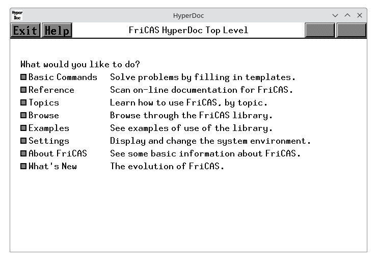
The HyperDoc root window page.
HyperDoc is the gateway to FriCAS. It’s both an on-line tutorial and an on-line reference manual. It also enables you to use FriCAS simply by using the mouse and filling in templates. HyperDoc is available to you if you are running FriCAS under the X Window System.
Pages usually have active areas, marked in this font (bold face). As you move the mouse pointer to an active area, the pointer changes from a filled dot to an open circle. The active areas are usually linked to other pages. When you click on an active area, you move to the linked page.
Most pages have a standard set of buttons at the top of the page. These are what they mean:

Click on this to get help. The button only appears if there is specific help for the page you are viewing. You can get general help for HyperDoc by clicking the help button on the home page.

Click here to go back one page. By clicking on this button repeatedly, you can go back several pages and then take off in a new direction.

Go back to the home page, that is, the page on which you started. Use HyperDoc to explore, to make forays into new topics. Don’t worry about how to get back. HyperDoc remembers where you came from. Just click on this button to return.

From the root window (the one that is displayed when you start the system) this button leaves the HyperDoc program, and it must be restarted if you want to use it again. From any other HyperDoc window, it just makes that one window go away. You must use this button to get rid of a window. If you use the window manager “Close” button, then all of HyperDoc goes away.
The buttons are not displayed if they are not applicable to the page you are viewing. For example, there is no
button on the top-level menu.
The following keyboard definitions are in effect throughout HyperDoc. See Section 3.3 on page 200 and Section 3.4 on page 200 for some contextual key definitions.
Display the main help page.
Same as , makes the window go away if you are not at the top-level window or quits the
HyperDoc facility if you are at the top-level.
Rereads the HyperDoc database, if necessary (for system developers).
Displays this information about key definitions.
Same as F3.
Scroll up one line.
Scroll down one line.
Scroll up one page.
Scroll down one page.
Whenever there is too much text to fit on a page, a scroll bar automatically appears along the right side.
With a scroll bar, your page becomes an aperture, that is, a window into a larger amount of text than can be displayed at one time. The scroll bar lets you move up and down in the text to see different parts. It also shows where the aperture is relative to the whole text. The aperture is indicated by a strip on the scroll bar.
Move the cursor with the mouse to the “down-arrow” at the bottom of the scroll bar and click. See that the aperture moves down one line. Do it several times. Each time you click, the aperture moves down one line. Move the mouse to the “up-arrow” at the top of the scroll bar and click. The aperture moves up one line each time you click.
Next move the mouse to any position along the middle of the scroll bar and click. HyperDoc attempts to move the top of the aperture to this point in the text.
You cannot make the aperture go off the bottom edge. When the aperture is about half the size of text, the lowest you can move the aperture is halfway down.
To move up or down one screen at a time, use the PageUp and PageDown keys on your keyboard. They move the visible part of the region up and down one page each time you press them.
If the HyperDoc page does not contain an input area (see Section 3.4 on page 200), you can also use the
Home and  and
 arrow keys to navigate. When you press the Home key, the screen is positioned at
the very top of the page. Use the
 and
 arrow keys to move the screen up and down one line at a time,
respectively.
Input areas are boxes where you can put data.
To enter characters, first move your mouse cursor to somewhere within the HyperDoc page. Characters that you type are inserted in front of the underscore. This means that when you type characters at your keyboard, they go into this first input area.
The input area grows to accommodate as many characters as you type. Use the Backspace key to erase
characters to the left. To modify what you type, use the right-arrow  and left-arrow keys
 and the
keys Insert, Delete, Home and End. These keys are found immediately on the right of the standard IBM
keyboard.
If you press the Home key, the cursor moves to the beginning of the line and if you press the End key, the cursor moves to the end of the line. Pressing Ctrl–End deletes all the text from the cursor to the end of the line.
A page may have more than one input area. Only one input area has an underscore cursor. When you first see a page, the top-most input area contains the cursor. To type information into another input area, use the Enter or Tab key to move from one input area to another. To move in the reverse order, use Shift–Tab.
You can also move from one input area to another using your mouse. Notice that each input area is active. Click on one of the areas. As you can see, the underscore cursor moves to that window.
Some pages have radio buttons and toggles. Radio buttons are a group of buttons like those on car radios: you can select only one at a time. Once you have selected a button, it appears to be inverted and contains a checkmark. To change the selection, move the cursor with the mouse to a different radio button and click.
A toggle is an independent button that displays some on/off state. When “on”, the button appears to be inverted and contains a checkmark. When “off”, the button is raised. Unlike radio buttons, you can set a group of them any way you like. To change toggle the selection, move the cursor with the mouse to the button and click.
A search string is used for searching some database. To learn about search strings, we suggest that you bring up the HyperDoc glossary. To do this from the top-level page of HyperDoc:
The glossary has an input area at its bottom. We review the various kinds of search strings you can enter to search the glossary.
The simplest search string is a word, for example, operation. A word only matches an entry having exactly that spelling. Enter the word operation into the input area above then click on Search. As you can see, operation matches only one entry, namely with operation itself.
Normally matching is insensitive to whether the alphabetic characters of your search string are in uppercase or lowercase. Thus operation and OperAtion both have the same effect.
You will very often want to use the wildcard “*” in your search string so as to match multiple entries in the list. The search key “*” matches every entry in the list. You can also use “*” anywhere within a search string to match an arbitrary substring. Try cat* for example: enter cat* into the input area and click on Search. This matches several entries.
You can use any number of wildcards in a search string as long as they are not adjacent. Try search strings such as *dom*. As you see, this search string matches domain, domain constructor, subdomain, and so on.
For more complicated searches, you can use “and”, “or”, and “not” with basic search strings; write logical expressions using these three operators just as in the FriCAS language. For example, domain or package matches the two entries domain and package. Similarly, dom* and *con* matches domain constructor and others. Also not *a* matches every entry that does not contain the letter a somewhere.
Use parentheses for grouping. For example, dom* and (not *con*) matches domain but not domain constructor.
There is no limit to how complex your logical expression can be. For example,
a* or b* or c* or d* or e* and (not *a*)
is a valid expression.
Many pages have FriCAS example commands. Each command has an active “button” along the left margin. When you click on this button, the output for the command is “pasted-in.” Click again on the button and you see that the pasted-in output disappears.
Maybe you would like to run an example? To do so, just click on any part of its text! When you do, the example line is copied into a new interactive FriCAS buffer for this HyperDoc page.
Sometimes one example line cannot be run before you run an earlier one. Don’t worry—HyperDoc automatically runs all the necessary lines in the right order!
The new interactive FriCAS buffer disappears when you leave HyperDoc. If you want to get rid of it beforehand, use the Cancel button of the X Window manager or issue the FriCAS system command )close.
You can control the appearance of HyperDoc while running under Version 11 of the X Window System by placing the following resources in the file .Xdefaults in your home directory. In what follows, font is any valid X11 font name (for example, Rom14) and color is any valid X11 color specification (for example, NavyBlue). For more information about fonts and colors, refer to the X Window documentation for your system.
This is the standard text font. The default value is "Rom14".
This is the standard text color. The default value is "black".
This is the font used for HyperDoc link buttons. The default value is "Bld14".
This is the color used for HyperDoc link buttons. The default value is "black".
This is the font used for active FriCAS commands. The default value is "Bld14".
This is the color used for active FriCAS commands. The default value is "black".
This is the font used for bold face. The default value is "Bld14".
This is the color used for bold face. The default value is "black".
This is the font used for FriCAS output in HyperDoc. This font must be fixed-width. The default
value is "Rom14".
This is the color used for FriCAS output in HyperDoc. The default value is "black".
This is the font used for italics. The default value is "Itl14".
This is the color used for italics. The default value is "black".
This is the color used as the background for input areas. The default value is "black".
This is the color used as the foreground for input areas. The default value is "white".
This is the color used for drawing border lines. The default value is "black".
This is the color used for the background of all windows. The default value is "white".
Note: In the past, resource names used the word Axiom instead of FriCAS.
In this chapter we discuss how to collect FriCAS statements and commands into files and then read the contents into the workspace. We also show how to display the results of your computations in several different styles including TeX, FORTRAN and monospace two-dimensional format.1
The printed version of this book uses the FriCAS TeX output formatter. When we demonstrate a particular output style, we will need to turn TeX formatting off and the output style on so that the correct output is shown in the text.
In this section we explain what an input file is and why you would want to know about it. We discuss where FriCAS looks for input files and how you can direct it to look elsewhere. We also show how to read the contents of an input file into the workspace and how to use the history facility to generate an input file from the statements you have entered directly into the workspace.
An input file contains FriCAS expressions and system commands. Anything that you can enter directly to FriCAS can be put into an input file. This is how you save input functions and expressions that you wish to read into FriCAS more than one time.
To read an input file into FriCAS, use the )read system command. For example, you can read a file in a particular directory by issuing
)read /spad/src/input/matrix.input
The “.input” is optional; this also works:
)read /spad/src/input/matrix
What happens if you just enter )read matrix.input or even )read matrix? FriCAS looks in your current working directory for input files that are not qualified by a directory name. Typically, this directory is the directory from which you invoked FriCAS. To change the current working directory, use the )cd system command. The command )cd by itself shows the current working directory. To change it to the src/input subdirectory for user “babar”, issue
)cd /u/babar/src/input
FriCAS looks first in this directory for an input file. If it is not found, it looks in the system’s directories, assuming you meant some input file that was provided with FriCAS.
If you have the FriCAS history facility turned on (which it is by default), you can save all the lines you have entered into the workspace by entering
)history )write
FriCAS tells you what input file to edit to see your statements. The file is in your home directory or in the directory you specified with )cd.
In Section 5.2 on page 248 we discuss using indentation in input files to group statements into blocks.
When FriCAS starts up, it tries to read the input file .fricas.input from your home directory. If there is no .fricas.input in your home directory, it reads the copy located in its own src/input directory. The file usually contains system commands to personalize your FriCAS environment. In the remainder of this section we mention a few things that users frequently place in their .fricas.input files.
In order to have FORTRAN output always produced from your computations, place the system command )set output fortran on in .fricas.input. If you do want to be prompted for confirmation when you issue the )quit system command, place )set quit protected in .fricas.input. If you then decide that you do not want to be prompted, issue )set quit unprotected. This is the default setting 2
To see the other system variables you can set, issue )set or use the HyperDoc Settings facility to view and change FriCAS system variables.
In this section we discuss how to start and stop the display of the different output formats and how to send the output to the screen or to a file. To fix ideas, we use FORTRAN output format for most of the examples.
You can use the )set output system command to toggle or redirect the different kinds of output. The name of the kind of output follows “output” in the command. The names are:
| fortran | for FORTRAN output. |
| algebra | for monospace two-dimensional mathematical output. |
| tex | for TeX output. |
| mathml | for MathML output. |
| texmacs | for TeXmacs output. |
For example, issue )set output fortran on to turn on FORTRAN format and issue )set output fortran off to turn it off. By default, algebra is on and all others are off. When output is started, it is sent to the screen. To send the output to a file, give the file name without directory or extension. FriCAS appends a file extension depending on the kind of output being produced. Issue this to redirect FORTRAN output to, for example, the file linalg.sfort.
)set output fortran linalg
FORTRAN output will be written to file linalg.sfort .
You must also turn on the creation of FORTRAN output. The above just says where it goes if it is created.
)set output fortran on
In what directory is this output placed? It goes into the directory from which you started FriCAS, or if you have used the )cd system command, the one that you specified with )cd. You should use )cd before you send the output to the file.
You can always direct output back to the screen by issuing this.
)set output fortran console
Let’s make sure FORTRAN formatting is off so that nothing we do from now on produces FORTRAN output.
)set output fortran off
We also delete the demonstrated output file we created.
)system rm linalg.sfort
You can abbreviate the words “on,” “off” and “console” to the minimal number of characters needed to
distinguish them. Because of this, you cannot send output to files called on.sfort, off.sfort, of.sfort,
console.sfort, consol.sfort and so on.
The width of the output on the page is set by )set output length for all formats except FORTRAN.
Use )set fortran fortlength to change the FORTRAN line length from its default value of
72.
This is the default output format for FriCAS. It is usually on when you start the system.
If it is not, issue this.
)set output algebra on
Since the printed version of this book (as opposed to the HyperDoc version) shows output produced by the TeX output formatter, let us temporarily turn off TeX output.
)set output tex off
Here is an example of what it looks like.
matrix [[i*x^i + j*%i*y^j for i in 1..2] for j in 3..4]
+ 3 3 2+ |3%i y + x 3%i y + 2x | | | | 4 4 2| +4%i y + x 4%i y + 2x +
Issue this to turn off this kind of formatting.
)set output algebra off
Turn TeX output on again.
)set output tex on
The characters used for the matrix brackets above are rather ugly. You get this character set when you issue )set output characters plain. This character set should be used when your machine or your version of FriCAS does not support Unicode character set. If your machine and your version of FriCAS support Unicode, issue )set output characters default to get better looking output.
FriCAS can produce TeX output for your expressions. The output is produced using macros from the LaTeX document preparation system by Leslie Lamport.3 The printed version of this book was produced using this formatter.
To turn on TeX output formatting, issue this.
)set output tex on
Here is an example of its output.
matrix [[i*x^i + j*%i*y^j for i in 1..2] for j in 3..4]
\begin{fricasmath}{1}
\begin{MATRIX}{2}3\TIMES \ImaginaryI \TIMES \SUPER{\SYMBOL{y}}{3}+\SYMBOL{x}&%
3\TIMES \ImaginaryI \TIMES \SUPER{\SYMBOL{y}}{3}+2\TIMES \SUPER{\SYMBOL{x}}{2%
}\\4\TIMES \ImaginaryI \TIMES \SUPER{\SYMBOL{y}}{4}+\SYMBOL{x}&4\TIMES %
\ImaginaryI \TIMES \SUPER{\SYMBOL{y}}{4}+2\TIMES \SUPER{\SYMBOL{x}}{2}%
\end{MATRIX}%
\end{fricasmath}
With the definition of the fricasmath environment as defined in fricasmath.sty this formats as
| (1) |
To turn TeX output formatting off, issue )set output tex off. The LaTeX macros in the output generated by FriCAS are generic. See the source file of TexFormat for appropriate definitions of these commands.
FriCAS can produce MathML format output for your expressions.
To turn MathML Format on, issue this.
)set output mathml on
Here is an example of its output.
x+sqrt(2) <math xmlns="http://www.w3.org/1998/Math/MathML" mathsize="big" display="block"> <mrow><mi>x</mi><mo>+</mo><msqrt><mrow><mn>2</mn></mrow></msqrt></mrow> </math>
To turn MathML Format output formatting off, issue this.
)set output mathml off
FriCAS can produce TeXmacs Scheme format output for your expressions. This is mostly useful for interfacing with TeXmacs.
To turn TeXmacs Format on, issue this.
)set output texmacs on
Here is an example of its output.
x+sqrt(2) scheme: (with "mode" "math" (concat (concat "x" ) "+" (sqrt (concat "2" ))) )
To turn TeXmacs Format output formatting off, issue this.
)set output texmacs off
In addition to turning FORTRAN output on and off and stating where the output should be placed, there are many options that control the appearance of the generated code. In this section we describe some of the basic options. Issue )set fortran to see a full list with their current settings.
The output FORTRAN expression usually begins in column 7. If the expression needs more than one line, the ampersand character “&” is used in column 6. Since some versions of FORTRAN have restrictions on the number of lines per statement, FriCAS breaks long expressions into segments with a maximum of 1320 characters (20 lines of 66 characters) per segment. If you want to change this, say, to 660 characters, issue the system command )set fortran explength 660. You can turn off the line breaking by issuing )set fortran segment off. Various code optimization levels are available. FORTRAN output is produced after you issue this.
)set output fortran on
For the initial examples, we set the optimization level to 0, which is the lowest level.
)set fortran optlevel 0
The output is usually in columns 7 through 72, although fewer columns are used in the following examples so that the output fits nicely on the page.
)set fortran fortlength 60
By default, the output goes to the screen and is displayed before the standard FriCAS two-dimensional
output. In this example, an assignment to the variable R1 was generated because this is the result of step
1.
(x+y)^3
Polynomial(Integer) Here is an example that illustrates the line breaking.
(x+y+z)^3
Note in the above examples that integers are generally converted to floating point numbers, except in exponents. This is the default behavior but can be turned off by issuing )set fortran ints2floats off. The rules governing when the conversion is done are:
These rules only govern integers in expressions. Numbers generated by FriCAS for DIMENSION statements are
also integers.
To set the type of generated FORTRAN data, use one of the following:
)set fortran defaulttype REAL )set fortran defaulttype INTEGER )set fortran defaulttype COMPLEX )set fortran defaulttype LOGICAL )set fortran defaulttype CHARACTER
When temporaries are created, they are given a default type of REAL. Also, the REAL versions of functions are used by default.
sin(x)
Expression(Integer) At optimization level 1, FriCAS removes common subexpressions.
)set fortran optlevel 1
(x+y+z)^3
Polynomial(Integer) This changes the precision to DOUBLE. Substitute single for double to return to single
precision.
)set fortran precision double
Complex constants display the precision.
2.3 + 5.6*%i
Complex(Float) The function names that FriCAS generates depend on the chosen precision.
sin %e
Expression(Integer) Reset the precision to single and look at these two examples again.
)set fortran precision single
2.3 + 5.6*%i
sin %e
Expression(Integer) Expressions that look like lists, streams, sets or matrices cause array code to be generated.
[x+1,y+1,z+1]
List(Polynomial(Integer)) A temporary variable is generated to be the name of the array. This may have to be changed in your particular application.
set[2,3,4,3,5]
Set(PositiveInteger) By default, the starting index for generated FORTRAN arrays is 0.
matrix [[2.3,9.7],[0.0,18.778]]
Matrix(Float) To change the starting index for generated FORTRAN arrays to be 1, issue this. This value
can only be 0 or 1.
)set fortran startindex 1
Look at the code generated for the matrix again.
matrix [[2.3,9.7],[0.0,18.778]]
This section describes more advanced facilities which are available to users who wish to generate Fortran code from within FriCAS. There are facilities to manipulate templates, store type information, and generate code fragments or complete programs.
A template is a skeletal program which is “fleshed out” with data when it is processed. It is a sequence of active and passive parts: active parts are sequences of FriCAS commands which are processed as if they had been typed into the interpreter; passive parts are simply echoed verbatim on the Fortran output stream.
Suppose, for example, that we have the following template, stored in the file “test.tem”:
-- A simple template
beginVerbatim
DOUBLE PRECISION FUNCTION F(X)
DOUBLE PRECISION X
endVerbatim
outputAsFortran("F",f)
beginVerbatim
RETURN
END
endVerbatim
The passive parts lie between the two tokens beginVerbatim and endVerbatim. There are two active statements: one which is simply a FriCAS ( --) comment, and one which produces an assignment to the current value of f. We could use it as follows:
(4) ->f := 4.0/(1+X^2) 4 (4) ------ 2 X + 1 (5) ->processTemplate "test.tem" DOUBLE PRECISION FUNCTION F(X) DOUBLE PRECISION X F=4.0D0/(X*X+1.0D0) RETURN END (5) "CONSOLE"
(A more reliable method of specifying the filename will be introduced below.) Note that the Fortran assignment F=4.0D0/(X*X+1.0D0) automatically converted 4.0 and 1 into DOUBLE PRECISION numbers; in general, the FriCAS Fortran generation facility will convert anything which should be a floating point object into either a Fortran REAL or DOUBLE PRECISION object. Which alternative is used is determined by the command
)set fortran precision
It is sometimes useful to end a template before the file itself ends (e.g. to allow the template to be tested incrementally or so that a piece of text describing how the template works can be included). It is of course possible to “comment-out” the remainder of the file. Alternatively, the single token endInput as part of an active portion of the template will cause processing to be ended prematurely at that point.
The processTemplate command comes in two flavours. In the first case, illustrated above, it takes one argument of domain FileName, the name of the template to be processed, and writes its output on the current Fortran output stream. In general, a filename can be generated from directory, name and extension components, using the operation filename, as in
processTemplate filename("","test","tem")
There is an alternative version of processTemplate, which takes two arguments (both of domain FileName). In this case the first argument is the name of the template to be processed, and the second is the file in which to write the results. Both versions return the location of the generated Fortran code as their result ("CONSOLE" in the above example).
It is sometimes useful to be able to mix active and passive parts of a line or statement. For example you might want to generate a Fortran Comment describing your data set. For this kind of application we provide three functions as follows:
So we could create our comment as follows:
m := matrix [[1,2,3],[4,5,6]]
fortranLiteralLine(concat ["C\ \ \ \ \ \ The\ Matrix\ has\ ", nrows(m)::String, "\ rows\ and\ ", ncols(m)::String, "\ columns"])$FortranTemplate
or, alternatively:
fortranLiteral("C\ \ \ \ \ \ The\ Matrix\ has\ ")$FortranTemplate
fortranLiteral(nrows(m)::String)$FortranTemplate
fortranLiteral("\ rows\ and\ ")$FortranTemplate
fortranLiteral(ncols(m)::String)$FortranTemplate
fortranLiteral("\ columns")$FortranTemplate
fortranCarriageReturn()$FortranTemplate
We should stress that these functions, together with the outputAsFortran function are the only sure ways of getting output to appear on the Fortran output stream. Attempts to use FriCAS commands such as output or writeline! may appear to give the required result when displayed on the console, but will give the wrong result when Fortran and algebraic output are sent to differing locations. On the other hand, these functions can be used to send helpful messages to the user, without interfering with the generated Fortran.
Sometimes it is useful to manipulate the Fortran output stream in a program, possibly without being aware of its current value. The main use of this is for gathering type declarations (see “Fortran Types” below) but it can be useful in other contexts as well. Thus we provide a set of commands to manipulate a stack of (open) output streams. Only one stream can be written to at any given time. The stack is never empty—its initial value is the console or the current value of the Fortran output stream, and can be determined using
topFortranOutputStack()$FortranOutputStackPackage
String (see below). The commands available to manipulate the stack are:
These commands are all part of FortranOutputStackPackage.
When generating code it is important to keep track of the Fortran types of the objects which we are generating. This is useful for a number of reasons, not least to ensure that we are actually generating legal Fortran code. The current type system is built up in several layers, and we shall describe each in turn.
This domain represents the simple Fortran datatypes: REAL, DOUBLE PRECISION, COMPLEX, LOGICAL, INTEGER, and CHARACTER. It is possible to coerce a String or Symbol into the domain, test whether two objects are equal, and also apply the predicate functions real? etc.
This domain represents “full” types: i.e., datatype plus array dimensions (where appropriate) plus whether or not the parameter is an external subprogram. It is possible to coerce an object of FortranScalarType into the domain or construct one from an element of FortranScalarType, a list of Polynomial Integers (which can of course be simple integers or symbols) representing its dimensions, and a Boolean declaring whether it is external or not. The list of dimensions must be empty if the Boolean is true. The functions scalarTypeOf, dimensionsOf and external? return the appropriate parts, and it is possible to get the various basic Fortran Types via functions like fortranReal. For example:
type:=construct(real,[i,10],false)$FortranType
or
type:=[real,[i,10],false]$FortranType
scalarTypeOf type
Union(fst: FortranScalarType, ...)
dimensionsOf type
external? type
fortranLogical()$FortranType
construct(integer,[],true)$FortranType
This domain creates and manipulates a symbol table for generated Fortran code. This is used by
FortranProgram to represent the types of objects in a subprogram. The commands available
are:
symbols := empty()$SymbolTable
declare!(X, fortranReal()$FortranType, symbols)
declare!(M,construct(real,[i,j],false)$FortranType,symbols)
declare!([i,j], fortranInteger()$FortranType, symbols)
symbols
fortranTypeOf(i,symbols)
typeList(real,symbols)
List(Union(name: Symbol, bounds: List(Union(S: Symbol, P: Polynomial(Integer)))))
printTypes symbols
This domain creates and manipulates one global symbol table to be used, for example, during template processing. It is also used when linking to external Fortran routines. The information stored for each subprogram (and the main program segment, where relevant) is:
Initially, any information provided is deemed to be for the main program segment. Issuing the following
command indicates that from now on all information refers to the subprogram F.
newSubProgram(F)$TheSymbolTable
It is possible to return to processing the main program segment by issuing the command:
endSubProgram()$TheSymbolTable
Symbol The following commands exist:
| declares the return type of the current subprogram |
|
|
|
|
| returns the return type of a subprogram |
|
|
|
|
| declares the argument list of the current subprogram |
|
|
|
|
| returns the argument list of a subprogram |
|
|
|
|
| provides type declarations for parameters of the current subprogram |
|
|
|
|
| returns the symbol table of a subprogram |
|
|
|
|
| produces the Fortran header for the current subprogram |
In addition there are versions of these commands which are parameterised by the name of a subprogram, and others parameterised by both the name of a subprogram and by an instance of TheSymbolTable.
newSubProgram(F)$TheSymbolTable
argumentList!(F, [X])$TheSymbolTable
returnType!(F,real)$TheSymbolTable
declare!(X,fortranReal(),F)$TheSymbolTable
printHeader(F)$TheSymbolTable
This section describes facilities for representing Fortran statements, and building up complete subprograms from them.
This domain is used to represent statements like x < y. Although these can be represented directly in FriCAS, it is a little cumbersome.
Instead we have a set of operations, such as LT to represent <, to let us build such statements. The available
constructors are:
So for example:
LT(x,y)$Switch
This domain represents code segments or operations: currently assignments, conditionals, blocks, comments, gotos, continues, various kinds of loops, and return statements. For example we can create quite a complicated conditional statement using assignments, and then turn it into Fortran code:
c := cond(LT(X,Y),assign(F,X),cond(GT(Y,Z),assign(F,Y),assign(F,Z))$FortranCode)$FortranCode
printCode c
The Fortran code is printed on the current Fortran output stream.
This domain is used to construct complete Fortran subprograms out of elements of FortranCode. It is parameterised by the name of the target subprogram (a Symbol), its return type (from Union(FortranScalarType,“void”)), its arguments (from List Symbol), and its symbol table (from SymbolTable). One can coerce elements of either FortranCode or Expression into it.
First of all we create a symbol table:
symbols := empty()$SymbolTable
SymbolTable Now put some type declarations into it:
declare!([X,Y],fortranReal()$FortranType,symbols)
FortranType Then (for convenience) we set up the particular instantiation of FortranProgram
FP := FortranProgram(F,real,[X,Y],symbols)
Type Create an object of type Expression(Integer):
asp := X*sin(Y)
Expression(Integer) Now coerce it into FP, and print its Fortran form:
outputAsFortran(asp::FP)
We can generate a FortranProgram using FortranCode. For example: Augment our symbol table:
declare!(Z,fortranReal()$FortranType,symbols)
FortranType prepare conditional:
cc := cond(LT(X,Y),assign(F,X),assign(F,Y))$FortranCode
FortranCode and transform the conditional expression we prepared earlier:
outputAsFortran([cc,returns()$FortranCode]::FP)
In this chapter we look at some of the basic components of the FriCAS language that you can use interactively. We show how to create a block of expressions, how to form loops and list iterations, how to modify the sequential evaluation of a block and how to use if-then-else to evaluate parts of your program conditionally. We suggest you first read the boxed material in each section and then proceed to a more thorough reading of the chapter.
A variable in FriCAS refers to a value. A variable has a name beginning with an uppercase or lowercase alphabetic character, “%”, or “!”. Successive characters (if any) can be any of the above, digits, or “?”. Case is distinguished. The following are all examples of valid, distinct variable names:
a tooBig? a1B2c3%!? A %j numberOfPoints beta6 %J numberofpoints
The “:=” operator is the immediate assignment operator. Use it to associate a value with a variable.
The syntax for immediate assignment for a single variable is
variable := expression
The value returned by an immediate assignment is the value of expression.
The right-hand side of the expression is evaluated, yielding 1. This value is then assigned to
a.
a := 1
PositiveInteger The right-hand side of the expression is evaluated, yielding 1. This value is then assigned to b.
Thus a and b both have the value 1 after the sequence of assignments.
b := a
PositiveInteger What is the value of b if a is assigned the value 2?
a := 2
PositiveInteger As you see, the value of b is left unchanged.
b
PositiveInteger This is what we mean when we say this kind of assignment is immediate; b has no dependency on a
after the initial assignment. This is the usual notion of assignment found in programming languages such as
C, PASCAL and FORTRAN.
FriCAS provides delayed assignment with “==”. This implements a delayed evaluation of the right-hand side and dependency checking.
Using a and b as above, these are the corresponding delayed assignments.
a == 1
b == a
The right-hand side of each delayed assignment is left unevaluated until the variables on the left-hand sides are evaluated. Therefore this evaluation and …
a
Compiling body of rule a to compute value of type PositiveInteger
PositiveInteger this evaluation seem the same as before.
b
Compiling body of rule b to compute value of type PositiveInteger
PositiveInteger If we change a to 2
a == 2
Compiled code for a has been cleared.
Compiled code for b has been cleared.
1 old definition(s) deleted for function or rule a
then a evaluates to 2, as expected, but
a
Compiling body of rule a to compute value of type PositiveInteger
PositiveInteger the value of b reflects the change to a.
b
Compiling body of rule b to compute value of type PositiveInteger
It is possible to set several variables at the same time by using a tuple of variables and a tuple of expressions.1
The syntax for multiple immediate assignments is
(  ,
 , …,
 ) := (
 ,
 , …,
 )
The value returned by an immediate assignment is the value of  .
This sets x to 1 and y to 2.
(x,y) := (1,2)
PositiveInteger Multiple immediate assignments are parallel in the sense that the expressions on the right are all evaluated before any assignments on the left are made. However, the order of evaluation of these expressions is undefined. You can use multiple immediate assignment to swap the values held by variables.
(x,y) := (y,x)
PositiveInteger x has the previous value of y.
x
PositiveInteger y has the previous value of x.
y
There is no syntactic form for multiple delayed assignments. See the discussion in Section 6.8 on page 313 about how FriCAS differentiates between delayed assignments and user functions of no arguments.
A block is a sequence of expressions evaluated in the order that they appear, except as modified by control
expressions such as break, return, iterate and if-then-else constructions. The value of a block is the
value of the expression last evaluated in the block.
To leave a block early, use “=>”. For example, i < 0 => x. The expression before the “=>” must evaluate to true
or false. The expression following the “=>” is the return value for the block.
A block can be constructed in two ways:
Only the first form is available if you are entering expressions directly to FriCAS. Both forms are available in .input files.
In .input files, blocks can also be written using piles. The examples throughout this book are assumed to come from .input files.
In this example, we assign a rational number to a using a block consisting of three expressions. This block is
written as a pile. Each expression in the pile has the same indentation, in this case two spaces to the right of
the first line.
a := i := gcd(234,672) i := 3*i^5 - i + 1 1 / i
Fraction(Integer) Here is the same block written on one line. This is how you are required to enter it at the input prompt.
a := (i := gcd(234,672); i := 3*i^5 - i + 1; 1 / i)
Fraction(Integer) Blocks can be used to put several expressions on one line. The value returned is that of the last expression.
(a := 1; b := 2; c := 3; [a,b,c])
FriCAS gives you two ways of writing a block and the preferred way in an .input file is to use a pile. Roughly speaking, a pile is a block whose constituent expressions are indented the same amount. You begin a pile by starting a new line for the first expression, indenting it to the right of the previous line. You then enter the second expression on a new line, vertically aligning it with the first line. And so on. If you need to enter an inner pile, further indent its lines to the right of the outer pile. FriCAS knows where a pile ends. It ends when a subsequent line is indented to the left of the pile or the end of the file.
Blocks can be used to perform several steps before an assignment (immediate or delayed) is made.
d := c := a^2 + b^2 sqrt(c * 1.3)
Float Blocks can be used in the arguments to functions. (Here h is assigned 2.1 + 3.5.)
h := 2.1 + 1.0 3.5
Float Here the second argument to eval is x = z, where the value of z is computed in the first line of the
block starting on the second line.
eval(x^2 - x*y^2, z := %pi/2.0 - exp(4.1) x = z )
Polynomial(Float) Blocks can be used in the clauses of if-then-else expressions (see Section 5.3 on page
254).
if h > 3.1 then 1.0 else (z := cos(h); max(z,0.5))
Float This is the pile version of the last block.
if h > 3.1 then 1.0 else z := cos(h) max(z,0.5)
Float Blocks can be nested.
a := (b := factorial(12); c := (d := eulerPhi(22); factorial(d));b+c)
PositiveInteger This is the pile version of the last block.
a := b := factorial(12) c := d := eulerPhi(22) factorial(d) b+c
Since c + d does equal 3628855, a has the value of c and the last line is never evaluated.
a := c := factorial 10 d := fibonacci 10 c + d = 3628855 => c d
Like many other programming languages, FriCAS uses the three keywords if, then and else to form
conditional expressions. The else part of the conditional is optional. The expression between the if and then
keywords is a predicate: an expression that evaluates to or is convertible to either true or false, that is, a
Boolean.
An if-then-else expression always returns a value. If the else clause is missing then the entire expression
returns the unique value of Void. If both clauses are present, the type of the value returned by if is obtained
by resolving the types of the values of the two clauses. See Section 2.10 on page 186 for more
information.
The predicate must evaluate to, or be convertible to, an object of type Boolean: true or false. By default, the equal sign = creates an equation.
This is an equation. In particular, it is an object of type Equation Polynomial Integer.
x + 1 = y
Equation(Polynomial(Integer)) However, for predicates in if expressions, FriCAS places a default target type of Boolean
on the predicate and equality testing is performed. Thus you need not qualify the “=” in any way. In other
contexts you may need to tell FriCAS that you want to test for equality rather than create an equation.
In those cases, use “@” and a target type of Boolean. See Section 2.9 on page 179 for more
information.
The compound symbol meaning “not equal” in FriCAS is ~=. This can be used directly without a package call
or a target specification. The expression a ~= b is directly translated into not (a = b).
Many other functions have return values of type Boolean. These include <, <=, >, >=, ~= and member?. By
convention, operations with names ending in “?” return Boolean values.
The usual rules for piles are suspended for conditional expressions. In .input files, the then and else
keywords can begin in the same column as the corresponding if but may also appear to the right. Each of the
following styles of writing if-then-else expressions is acceptable:
if i>0 then output("positive") else output("nonpositive")
if i > 0 then output("positive")
else output("nonpositive")
if i > 0 then output("positive")
else output("nonpositive")
if i > 0
then output("positive")
else output("nonpositive")
if i > 0
then output("positive")
else output("nonpositive")
A block can follow the then or else keywords. In the following two assignments to a, the then and else
clauses each are followed by two-line piles. The value returned in each is the value of the second
line.
a := if i > 0 then j := sin(i * pi()) exp(j + 1/j) else j := cos(i * 0.5 * pi()) log(abs(j)^5 + 1) a := if i > 0 then j := sin(i * pi()) exp(j + 1/j) else j := cos(i * 0.5 * pi()) log(abs(j)^5 + 1)
These are both equivalent to the following:
a := if i > 0 then (j := sin(i * pi()); exp(j + 1/j)) else (j := cos(i * 0.5 * pi()); log(abs(j)^5 + 1))
A loop is an expression that contains another expression, called the loop body, which is to be evaluated zero or
more times. All loops contain the repeat keyword and return the unique value of Void. Loops can contain
inner loops to any depth.
FriCAS tries to determine completely the type of every object in a loop and then to translate the loop body to LISP or even to machine code. This translation is called compilation.
If FriCAS decides that it cannot compile the loop, it issues a message stating the problem and then the following message:
We will attempt to step through and interpret the code.
It is still possible that FriCAS can evaluate the loop but in interpret-code mode. See Section 6.10 on page 318 where this is discussed in terms of compiling versus interpreting functions.
A return expression is used to exit a function with a particular value. In particular, if a return is in a loop
within the function, the loop is terminated whenever the return is evaluated. Suppose we start with
this.
f() == i := 1 repeat if factorial(i) > 1000 then return i i := i + 1
When factorial(i) is big enough, control passes from inside the loop all the way outside the function,
returning the value of i (or so we think).
f()
Compiling function f with type () -> Void
What went wrong? Isn’t it obvious that this function should return an integer? Well, FriCAS makes no attempt to analyze the structure of a loop to determine if it always returns a value because, in general, this is impossible. So FriCAS has this simple rule: the type of the function is determined by the type of its body, in this case a block. The normal value of a block is the value of its last expression, in this case, a loop. And the value of every loop is the unique value of Void! So the return type of f is Void.
There are two ways to fix this. The best way is for you to tell FriCAS what the return type of f is. You do
this by giving f a declaration f: () prior to calling for its value. This tells FriCAS: “trust
me—an integer is returned.” We’ll explain more about this in the next chapter. Another clumsy way is to add
a dummy expression as follows.
 Integer
Since we want an integer, let’s stick in a dummy final expression that is an integer and will never be evaluated.
f() == i := 1 repeat if factorial(i) > 1000 then return i i := i + 1 0
Compiled code for f has been cleared.
1 old definition(s) deleted for function or rule f
When we try f again we get what we wanted. See Section 6.15 on page 342 for more information.
f()
Compiling function f with type () -> NonNegativeInteger
The break keyword is often more useful in terminating a loop. A break causes control to transfer to the
expression immediately following the loop. As loops always return the unique value of Void, you cannot
return a value with break. That is, break takes no argument.
This example is a modification of the last example in the previous section. Instead of using return, we’ll use
break.
f() == i := 1 repeat if factorial(i) > 1000 then break i := i + 1 i
The loop terminates when factorial(i) gets big enough, the last line of the function evaluates to the
corresponding “good” value of i, and the function terminates, returning that value.
f()
Compiling function f with type () -> PositiveInteger
PositiveInteger You can only use break to terminate the evaluation of one loop. Let’s consider a loop within a
loop, that is, a loop with a nested loop. First, we initialize two counter variables.
(i,j) := (1, 1)
PositiveInteger Nested loops must have multiple break expressions at the appropriate nesting level. How would
you rewrite this so (i + j)> 10 is only evaluated once?
repeat repeat if (i + j) > 10 then break j := j + 1 if (i + j) > 10 then break i := i + 1
Compare the following two loops:
i := 1 i := 1 repeat repeat i := i + 1 i := i + 1 i > 3 => i if i > 3 then break output(i) output(i)
In the example on the left, the values  and
 for
i are displayed but then the “=>” does not allow control
to reach the call to output again. The loop will not terminate until you run out of space or interrupt the
execution. The variable i will continue to be incremented because the “=>” only means to leave the block, not
the loop.
In the example on the right, upon reaching  , the
break will be executed, and both the block and the loop
will terminate. This is one of the reasons why both “=>” and break are provided. Using a while clause (see
below) with the “=>” lets you simulate the action of break.
Here we give four examples of repeat loops that terminate when a value exceeds a given bound.
First, initialize i as the loop counter.
i := 0
NonNegativeInteger Here is the first loop. When the square of i exceeds 100, the loop terminates.
repeat i := i + 1 if i^2 > 100 then break
Upon completion, i should have the value 11.
i
NonNegativeInteger Do the same thing except use “=>” instead of an if-then expression.
i := 0
repeat i := i + 1 i^2 > 100 => break
i
NonNegativeInteger As a third example, we use a simple loop to compute n!.
(n, i, f) := (100, 1, 1)
PositiveInteger Use i as the iteration variable and f to compute the factorial.
repeat if i > n then break f := f * i i := i + 1
Look at the value of f.
f
PositiveInteger Finally, we show an example of nested loops. First define a four by four matrix.
m := matrix [[21,37,53,14], [8,-24,22,-16], [2,10,15,14], [26,33,55,-13]]
Matrix(Integer) Next, set row counter r and column counter c to  . Note: if we were writing a function,
these would all be local variables rather than global workspace variables.
(r, c) := (1, 1)
PositiveInteger Also, let lastrow and lastcol be the final row and column index.
(lastrow, lastcol) := (nrows(m), ncols(m))
PositiveInteger Scan the rows looking for the first negative element. We remark that you can reformulate this
example in a better, more concise form by using a for clause with repeat. See Section 5.4.8 on page 271 for
more information.
repeat if r > lastrow then break c := 1 repeat if c > lastcol then break if elt(m,r,c) < 0 then output [r, c, elt(m,r,c)] r := lastrow break -- don’t look any further c := c + 1 r := r + 1
[2, 2, - 24]
FriCAS provides an iterate expression that skips over the remainder of a loop body and starts the next loop
iteration. We first initialize a counter.
i := 0
NonNegativeInteger Display the even integers from 2 to 5.
repeat i := i + 1 if i > 5 then break if odd?(i) then iterate output(i)
2
4
The repeat in a loop can be modified by adding one or more while clauses. Each clause contains a predicate
immediately following the while keyword. The predicate is tested before the evaluation of the
body of the loop. The loop body is evaluated whenever the predicates in a while clause are all
true.
The syntax for a simple loop using while is
while predicate repeat loopBody
The predicate is evaluated before loopBody is evaluated. A while loop terminates immediately when predicate
evaluates to false or when a break or return expression is evaluated in loopBody. The value returned by the
loop is the unique value of Void.
Here is a simple example of using while in a loop. We first initialize the counter.
i := 1
PositiveInteger The steps involved in computing this example are (1) set i to 1, (2) test the condition i < 1 and
determine that it is not true, and (3) do not evaluate the loop body and therefore do not display
"hello".
while i < 1 repeat output "hello" i := i + 1
If you have multiple predicates to be tested use the logical and operation to separate them. FriCAS evaluates
these predicates from left to right.
(x, y) := (1, 1)
while x < 4 and y < 10 repeat output [x,y] x := x + 1 y := y + 2
[1, 1]
[2, 3]
[3, 5]
A break expression can be included in a loop body to terminate a loop even if the predicate in any while
clauses are not false.
(x, y) := (1, 1)
PositiveInteger This loop has multiple while clauses and the loop terminates before any one of their conditions
evaluates to false.
while x < 4 while y < 10 repeat if x + y > 7 then break output [x,y] x := x + 1 y := y + 2
[1, 1]
[2, 3]
Here’s a different version of the nested loops that looked for the first negative element in a matrix.
m := matrix [[21,37,53,14], [8,-24,22,-16], [2,10,15,14], [26,33,55,-13]]
Matrix(Integer) Initialize the row index to 1 and get the number of rows and columns. If we were writing a
function, these would all be local variables.
r := 1
(lastrow, lastcol) := (nrows(m), ncols(m))
PositiveInteger Scan the rows looking for the first negative element.
while r <= lastrow repeat c := 1 -- index of first column while c <= lastcol repeat if elt(m,r,c) < 0 then output [r, c, elt(m,r,c)] r := lastrow break -- don’t look any further c := c + 1 r := r + 1
[2, 2, - 24]
FriCAS provides the for and in keywords in repeat loops, allowing you to iterate across all elements of a list,
or to have a variable take on integral values from a lower bound to an upper bound. We shall refer to these
modifying clauses of repeat loops as for clauses. These clauses can be present in addition to while clauses.
As with all other types of repeat loops, break can be used to prematurely terminate the evaluation of the
loop.
The syntax for a simple loop using for is
for iterator repeat loopBody
The iterator has several forms. Each form has an end test which is evaluated before loopBody is evaluated. A
for loop terminates immediately when the end test succeeds (evaluates to true) or when a break or
return expression is evaluated in loopBody. The value returned by the loop is the unique value of
Void.
If for is followed by a variable name, the in keyword and then an integer segment of the form n..m, the end
test for this loop is the predicate i > m. The body of the loop is evaluated m-n+1 times if this number
is greater than 0. If this number is less than or equal to 0, the loop body is not evaluated at
all.
The variable i has the value n, n+1, ..., m for successive iterations of the loop body. The loop variable is a
local variable within the loop body: its value is not available outside the loop body and its value and
type within the loop body completely mask any outer definition of a variable with the same
name.
This loop prints the values of  ,
 , and
 :
for i in 10..12 repeat output(i^3)
1000
1331
1728
Here is a sample list.
a := [1,2,3]
List(PositiveInteger) Iterate across this list, using “.” to access the elements of a list and the # operation to count its elements.
for i in 1..#a repeat output(a.i)
1
2
3
This type of iteration is applicable to anything that uses “.”. You can also use it with functions that use
indices to extract elements. Define m to be a matrix.
m := matrix [[1,2],[4,3],[9,0]]
Matrix(NonNegativeInteger) Display the rows of m.
for i in 1..nrows(m) repeat output row(m,i)
[1, 2]
[4, 3]
[9, 0]
You can use iterate with for-loops. Display the even integers in a segment.
for i in 1..5 repeat if odd?(i) then iterate output(i)
2
4
See ‘Segment’ on page 1263 for more information about segments.
By default, the difference between values taken on by a variable in loops such as for i in n..m repeat ... is  .
It is possible to supply another, possibly negative, step value by using the
by keyword along with for and in.
Like the upper and lower bounds, the step value following the by keyword must be an integer. Note that the
loop for i in 1..2 by 0 repeat output(i) will not terminate by itself, as the step value does not change the
index from its initial value of  .
This expression displays the odd integers between two bounds.
for i in 1..5 by 2 repeat output(i)
1
3
5
Use this to display the numbers in reverse order.
for i in 5..1 by -2 repeat output(i)
5
3
1
If the value after the “..” is omitted, the loop has no end test. A potentially infinite loop is thus created. The
variable is given the successive values n, n+1, n+2, ... and the loop is terminated only if a break or return
expression is evaluated in the loop body. However you may also add some other modifying clause on the
repeat (for example, a while clause) to stop the loop.
This loop displays the integers greater than or equal to 15 and less than the first prime greater than
15.
for i in 15.. while not prime?(i) repeat output(i)
15
16
Another variant of the for loop has the form:
for x in list repeat loopBody
This form is used when you want to iterate directly over the elements of a list. In this form of the for loop,
the variable x takes on the value of each successive element in l. The end test is most simply stated in
English: “are there no more x in l?”
If l is this list,
l := [0,-5,3]
List(Integer) display all elements of l, one per line.
for x in l repeat output(x)
0
- 5
3
Since the list constructing expression expand [n..m] creates the list
[n, n+1, ..., m]2,
you might be tempted to think that the loops
for i in n..m repeat output(i)
and
for x in expand [n..m] repeat output(x)
are equivalent. The second form first creates the list expand [n..m] (no matter how large it might be) and
then does the iteration. The first form potentially runs in much less space, as the index variable i is simply
incremented once per loop and the list is not actually created. Using the first form is much more efficient. Of
course, sometimes you really want to iterate across a specific list. This displays each of the factors of
2400000.
for f in factors(factor(2400000)) repeat output(f)
[factor = 2, exponent = 8]
[factor = 3, exponent = 1]
[factor = 5, exponent = 5]
A for loop can be followed by a “|” and then a predicate. The predicate qualifies the use of the values from
the iterator following the for. Think of the vertical bar “|” as the phrase “such that.” This loop expression
prints out the integers n in the given segment such that n is odd.
for n in 0..4 | odd? n repeat output n
1
3
A for loop can also be written
for iterator | predicate repeat loopBody
which is equivalent to:
for iterator repeat if predicate then loopBody else iterate
The predicate need not refer only to the variable in the for clause: any variable in an outer scope can be part
of the predicate. In this example, the predicate on the inner for loop uses i from the outer loop and the j
from the for clause that it directly modifies.
for i in 1..50 repeat for j in 1..50 | factorial(i+j) < 25 repeat output [i,j]
[1, 1]
[1, 2]
[1, 3]
[2, 1]
[2, 2]
[3, 1]
The last example of the previous section gives an example of nested iteration: a loop is contained in another loop. Sometimes you want to iterate across two lists in parallel, or perhaps you want to traverse a list while incrementing a variable.
The general syntax of a repeat loop is

 …
 repeat loopBody
where each iterator is either a for or a while clause. The loop terminates immediately when the end test of
any iterator succeeds or when a break or return expression is evaluated in loopBody. The value returned by
the loop is the unique value of Void.
Here we write a loop to iterate across two lists, computing the sum of the pairwise product of elements. Here is the first list.
l := [1,3,5,7]
List(PositiveInteger) And the second.
m := [100,200]
List(PositiveInteger) The initial value of the sum counter.
sum := 0
NonNegativeInteger The last two elements of l are not used in the calculation because m has two fewer elements than
l.
for x in l for y in m repeat sum := sum + x*y
Display the “dot product.”
sum
Next, we write a loop to compute the sum of the products of the loop elements with their positions in the loop.
l := [2,3,5,7,11,13,17,19,23,29,31,37]
List(PositiveInteger) The initial sum.
sum := 0
NonNegativeInteger Here looping stops when the list l is exhausted, even though the for i in 0.. specifies no
terminating condition.
for i in 0.. for x in l repeat sum := i * x
Display this weighted sum.
sum
When “|” is used to qualify any of the for clauses in a parallel iteration, the variables in the predicates can
be from an outer scope or from a for clause in or to the left of a modified clause.
This is correct:
for i in 1..10 repeat for j in 200..300 | odd? (i+j) repeat output [i,j]
This is not correct since the variable j has not been defined outside the inner loop.
for i in 1..10 | odd? (i+j) repeat -- wrong, j not defined for j in 200..300 repeat output [i,j]
This example shows that it is possible to mix several of the forms of repeat modifying clauses on a
loop.
for i in 1..10 for j in 151..160 | odd? j while i + j < 160 repeat output [i,j]
[1, 151]
[3, 153]
Here are useful rules for composing loop expressions:
while predicates can only refer to variables that are global (or in an outer scope) or that are
defined in for clauses to the left of the predicate.
for clause and can only
refer to variables that are global (or in an outer scope) or defined in the modified for clause or
any for clause to the left.
All of what we did for loops in Section 5.4 on page 258 can be transformed into expressions that
create lists and streams. The repeat, break or iterate words are not used but all the other
ideas carry over. Before we give you the general rule, here are some examples which give you the
idea.
This creates a simple list of the integers from 1 to 10.
mylist := [i for i in 1..10]
List(PositiveInteger) Create a stream of the integers greater than or equal to 1.
mystream := [i for i in 1..]
Stream(PositiveInteger) This is a list of the prime integers between 1 and 10, inclusive.
[i for i in 1..10 | prime? i]
List(PositiveInteger) This is a stream of the prime integers greater than or equal to 1.
[i for i in 1.. | prime? i]
Stream(PositiveInteger) This is a list of the integers between 1 and 10, inclusive, whose squares are less than
700.
[i for i in 1..10 while i*i < 700]
List(PositiveInteger) This is a stream of the integers greater than or equal to 1 whose squares are less than
700.
[i for i in 1.. while i*i < 700]
Got the idea? Here is the general rule.
The general syntax of a collection is
[ collectExpression 
 …
 ]
where each  is either a
for or a while clause. The loop terminates immediately when the end test of
any  succeeds or when a
return expression is evaluated in collectExpression. The value
returned by the collection is either a list or a stream of elements, one for each iteration of the
collectExpression.
Be careful when you use while to create a stream. By default, FriCAS tries to compute and display the first
ten elements of a stream. If the while condition is not satisfied quickly, FriCAS can spend a long (possibly
infinite) time trying to compute the elements. Use )set streams calculate to change the default to
something else. This also affects the number of terms computed and displayed for power series.
For the purposes of this book, we have used this system command to display fewer than ten
terms. Use nested iterators to create lists of lists which can then be given as an argument to
matrix.
matrix [[x^i+j for i in 1..3] for j in 10..12]
Matrix(Polynomial(Integer)) You can also create lists of streams, streams of lists and streams of streams. Here is a stream of streams.
[[i/j for i in j+1..] for j in 1..]
Stream(Stream(Fraction(Integer))) You can use parallel iteration across lists and streams to create new lists.
[i/j for i in 3.. by 10 for j in 2..]
Stream(Fraction(Integer)) Iteration stops if the end of a list or stream is reached.
[i^j for i in 1..7 for j in 2.. ]
Stream(Integer) As with loops, you can combine these modifiers to make very complicated conditions.
[[[i,j] for i in 10..15 | prime? i] for j in 17..22 | j = squareFreePart j]
List(List(List(PositiveInteger)))
See ‘List’ on page 1074 and ‘Stream’ on page 1300 for more information on creating and manipulating lists and streams, respectively.
We conclude this chapter with an example of the creation and manipulation of infinite streams of prime integers. This might be useful for experiments with numbers or other applications where you are using sequences of primes over and over again. As for all streams, the stream of primes is only computed as far out as you need. Once computed, however, all the primes up to that point are saved for future reference.
Two useful operations provided by the FriCAS library are prime? and nextPrime. A straight-forward way to
create a stream of prime numbers is to start with the stream of positive integers [2,..] and filter out those
that are prime. Create a stream of primes.
primes : Stream Integer := [i for i in 2.. | prime? i]
Stream(Integer) A more elegant way, however, is to use the stream operation from Stream. Given an initial
value a and a function f, stream constructs the stream [a, f(a), f(f(a)), ...]. This function gives you the
quickest method of getting the stream of primes. This is how you use stream to generate an infinite stream of
primes.
primes := stream(nextPrime,2)
Stream(Integer) Once the stream is generated, you might only be interested in primes starting at a particular value.
smallPrimes := [p for p in primes | p > 1000]
Stream(Integer) Here are the first 11 primes greater than 1000.
[p for p in smallPrimes for i in 1..11]
Stream(Integer) Here is a stream of primes between 1000 and 1200.
[p for p in smallPrimes while p < 1200]
Stream(Integer) To get these expanded into a finite stream, you call complete on the stream.
complete %
Stream(Integer) Twin primes are consecutive odd number pairs which are prime. Here is the stream of twin primes.
twinPrimes := [[p,p+2] for p in primes | prime?(p + 2)]
Stream(List(Integer)) Since we already have the primes computed we can avoid the call to prime? by using a double iteration. This time we’ll just generate a stream of the first of the twin primes.
firstOfTwins:= [p for p in primes for q in rest primes | q=p+2]
Let’s try to compute the infinite stream of triplet primes, the set of primes p such that [p,p+2,p+4] are
primes. For example, [3,5,7] is a triple prime. We could do this by a triple for iteration. A more
economical way is to use firstOfTwins. This time however, put a semicolon at the end of the
line.
Put a semicolon at the end so that no elements are computed.
firstTriplets := [p for p in firstOfTwins for q in rest firstOfTwins | q = p+2];
What happened? As you know, by default FriCAS displays the first ten elements of a stream when you first display it. And, therefore, it needs to compute them! If you want no elements computed, just terminate the expression by a semicolon (“;”).3
Compute the first triplet prime.
firstTriplets.1
If you want to compute another, just ask for it. But wait a second! Given three consecutive odd integers, one of them must be divisible by 3. Thus there is only one triplet prime. But suppose that you did not know this and wanted to know what was the tenth triplet prime.
firstTriplets.10
To compute the tenth triplet prime, FriCAS first must compute the second, the third, and so on. But since there isn’t even a second triplet prime, FriCAS will compute forever. Nonetheless, this effort can produce a useful result. After waiting a bit, hit Ctrl–c. The system responds as follows.
>> System error: Console interrupt. You are being returned to the top level of the interpreter.
Let’s say that you want to know how many primes have been computed. Issue
numberOfComputedEntries primes
and, for this discussion, let’s say that the result is 2045. How big is the  prime?
primes.2045
What you have learned is that there are no triplet primes between 5 and 17837. Although this result is well known (some might even say trivial), there are many experiments you could make where the result is not known. What you see here is a paradigm for testing of hypotheses. Here our hypothesis could have been: “there is more than one triplet prime.” We have tested this hypothesis for 17837 cases. With streams, you can let your machine run, interrupt it to see how far it has progressed, then start it up and let it continue from where it left off.
In this chapter we show you how to write functions and macros, and we explain how FriCAS looks for and applies them. We show some simple one-line examples of functions, together with larger ones that are defined piece-by-piece or through the use of piles.
A function is a program to perform some computation. Most functions have names so that it is easy to refer to them. A simple example of a function is one named abs which computes the absolute value of an integer. This is a use of the “absolute value” library function for integers.
abs(-8)
PositiveInteger This is an unnamed function that does the same thing, using the “maps-to” syntax “+->” that we discuss in Section 6.17 on page 357.
(x +-> if x < 0 then -x else x)(-8)
PositiveInteger Functions can be used alone or serve as the building blocks for larger programs. Usually they return a value that you might want to use in the next stage of a computation, but not always (for example, see ‘Exit’ on page 845 and ‘Void’ on page 1374). They may also read data from your keyboard, move information from one place to another, or format and display results on your screen.
In FriCAS, as in mathematics, functions are usually parameterized. Each time you call (some people say apply or invoke) a function, you give values to the parameters (variables). Such a value is called an argument of the function. FriCAS uses the arguments for the computation. In this way you get different results depending on what you “feed” the function.
Functions can have local variables or refer to global variables in the workspace. FriCAS can often compile functions so that they execute very efficiently. Functions can be passed as arguments to other functions.
Macros are textual substitutions. They are used to clarify the meaning of constants or expressions and to be templates for frequently used expressions. Macros can be parameterized but they are not objects that can be passed as arguments to functions. In effect, macros are extensions to the FriCAS expression parser.
A macro provides general textual substitution of an FriCAS expression for a name. You can think of a macro as being a generalized abbreviation. You can only have one macro in your workspace with a given name, no matter how many arguments it has.
The two general forms for macros are
macro name == body
macro name(arg1,...) == body
where the body of the macro can be any FriCAS expression.
For example, suppose you decided that you like to use df for D. You define the macro df like
this.
macro df == D
Whenever you type df, the system expands it to D.
df(x^2 + x + 1,x)
Polynomial(Integer) Macros can be parameterized and so can be used for many different kinds of objects.
macro ff(x) == x^2 + 1
Apply it to a number, a symbol, or an expression.
ff z
Polynomial(Integer) Macros can also be nested, but you get an error message if you run out of space because of an infinite nesting loop.
macro gg(x) == ff(2*x - 2/3)
This new macro is fine as it does not produce a loop.
gg(1/w)
Fraction(Polynomial(Integer)) This, however, loops since gg is defined in terms of ff.
macro ff(x) == gg(-x)
The body of a macro can be a block.
macro next == (past := present; present := future; future := past + present)
Before entering next, we need values for present and future.
present : Integer := 0
future : Integer := 1
Integer Repeatedly evaluating next produces the next Fibonacci number.
next
Integer And the next one.
next
Integer Here is the infinite stream of the rest of the Fibonacci numbers.
[next for i in 1..]
Stream(Integer) Bundle all the above lines into a single macro.
macro fibStream == present : Integer := 1 future : Integer := 1 [next for i in 1..] where macro next == past := present present := future future := past + present
Use concat to start with the first two Fibonacci numbers.
concat([1,1],fibStream)
Stream(Integer) An easier way to compute these numbers is to use the library operation fibonacci.
[fibonacci i for i in 1..]
Each name in your workspace can refer to a single object. This may be any kind of object including a function. You can use interactively any function from the library or any that you define in the workspace. In the library, the same name can have many functions, but you can have only one function with a given name, although it can have any number of arguments that you choose.
If you define a function in the workspace that has the same name and number of arguments as one in the library, then your definition takes precedence. In fact, to get the library function you must package-call it (see Section 2.9 on page 179).
To use a function in FriCAS, you apply it to its arguments. Most functions are applied by entering the name of the function followed by its argument or arguments.
factor(12)
Factored(Integer) Some functions like + have infix operators as names.
3 + 4
PositiveInteger The function + has two arguments. When you give it more than two arguments, FriCAS groups
the arguments to the left. This expression is equivalent to (1 + 2)+ 7.
1 + 2 + 7
All operations, including infix operators, can be written in prefix form, that is, with the operation name
followed by the arguments in parentheses. For example, 2 + 3 can alternatively be written as +(2,3). But
+(2,3,4) is an error since + takes only two arguments.
Prefix operations are generally applied before the infix operation. Thus factorial 3 + 1 means
factorial(3)+ 1 producing 7, and - 2 + 5 means (-2)+ 5 producing 3. An example of a prefix operator is prefix
-. For example, - 2 + 5 converts to (- 2)+ 5 producing the value 3. Any prefix function taking two arguments can
be written in an infix manner by putting an ampersand (“&”) before the name. Thus D(2*x,x) can be written
as 2*x &D x returning 2.
Every function in FriCAS is identified by a name and
type.1
The type of a function is always a mapping of the form Source where  Target
Source and Target are
types. To enter a type from the keyboard, enter the arrow by using a hyphen “-” followed by a greater-than
sign “>”, e.g. Integer
Let’s go back to +. There are many + functions in the FriCAS library: one for integers, one for floats, another for rational numbers, and so on. These + functions have different types and thus are different functions. You’ve seen examples of this overloading before—using the same name for different functions. Overloading is the rule rather than the exception. You can add two integers, two polynomials, two matrices or two power series. These are all done with the same function name but with different functions.
In Section 2.3 on page 146 we discussed how to declare a variable to restrict the kind of values that can be assigned to it. In this section we show how to declare a variable that refers to function objects.
A function is an object of type
Source Type
where Source and Target can be any type. A common type for Source is ( , …,
 ), to indicate a
function of
n arguments.
If g takes an Integer, a Float and another Integer, and returns a String, the declaration is written this
way.
g: (Integer,Float,Integer) -> String
The types need not be written fully; using abbreviations, the above declaration is:
g: (INT,FLOAT,INT) -> STRING
It is possible for a function to take no arguments. If h takes no arguments but returns a Polynomial
Integer, any of the following declarations is acceptable.
h: () -> POLY INT
h: () -> Polynomial INT
h: () -> POLY Integer
Functions can also be declared when they are being defined. The syntax for combined declaration/definition is:
functionName( :
 , …,
 :
 ): functionReturnType
The following definition fragments show how this can be done for the functions g and h above.
g(arg1: INT, arg2: FLOAT, arg3: INT): STRING == ... h(): POLY INT == ...
A current restriction on function declarations is that they must involve fully specified types (that is, cannot include modes involving explicit or implicit “?”). For more information on declaring things in general, see Section 2.3 on page 146.
As you use FriCAS, you will find that you will write many short functions to codify sequences of operations that you often perform. In this section we write some simple one-line functions.
This is a simple recursive factorial function for positive integers.
fac n == if n < 3 then n else n * fac(n-1)
fac 10
Compiling function fac with type Integer -> Integer
PositiveInteger This function computes 1 + 1/2 + 1/3 + ... + 1/n.
s n == reduce(+,[1/i for i in 1..n])
s 50
Compiling function s with type PositiveInteger -> Fraction(Integer)
Fraction(Integer) This function computes a Mersenne number, several of which are prime.
mersenne i == 2^i - 1
If you type mersenne, FriCAS shows you the function definition.
mersenne
FunctionCalled(mersenne) Generate a stream of Mersenne numbers.
[mersenne i for i in 1..]
Compiling function mersenne with type PositiveInteger -> Integer
Stream(Integer) Create a stream of those values of i such that mersenne(i) is prime.
mersenneIndex := [n for n in 1.. | prime?(mersenne(n))]
Stream(PositiveInteger) Finally, write a function that returns the  Mersenne prime.
mersennePrime n == mersenne mersenneIndex(n)
mersennePrime 5
Compiling function mersennePrime with type PositiveInteger -> Integer
If you declare the type of a function, you can apply it to any data that can be converted to the source type of the function.
Define f with type Integer
f(x: Integer): Integer == x + 1
Function declaration f : Integer -> Integer has been added to workspace.
The function f can be applied to integers, …
f 9
Compiling function f with type Integer -> Integer
PositiveInteger and to values that convert to integers, …
f(-2.0)
Integer but not to values that cannot be converted to integers.
f(2/3)
Conversion failed in the compiled user function f .
Cannot convert the value from type Fraction(Integer) to Integer .
To make the function over a wide range of types, do not declare its type. Give the same definition with no declaration.
g x == x + 1
If x + 1 makes sense, you can apply g to x.
g 9
Compiling function g with type PositiveInteger -> PositiveInteger
PositiveInteger A version of g with different argument types gets compiled for each new kind of argument used.
g(2/3)
Compiling function g with type Fraction(Integer) -> Fraction(Integer)
Fraction(Integer) Here x+1 for x = "fricas" makes no sense.
g("fricas")
There are 13 exposed and 13 unexposed library operations named + having 2 argument(s) but none was determined to be applicable. Use HyperDoc Browse, or issue )display op + to learn more about the available operations. Perhaps package-calling the operation or using coercions on the arguments will allow you to apply the operation.
Cannot find a definition or applicable library operation named + with argument type(s) String PositiveInteger Perhaps you should use "@" to indicate the required return type, or "$" to specify which version of the function you need.
FriCAS will attempt to step through and interpret the code.
There are 13 exposed and 13 unexposed library operations named + having 2 argument(s) but none was determined to be applicable. Use HyperDoc Browse, or issue )display op + to learn more about the available operations. Perhaps package-calling the operation or using coercions on the arguments will allow you to apply the operation.
Cannot find a definition or applicable library operation named + with argument type(s) String PositiveInteger Perhaps you should use "@" to indicate the required return type, or "$" to specify which version of the function you need.
As you will see in Chapter 12, FriCAS has a formal idea of categories for what “makes sense.”
A function is an object that you can create, manipulate, pass to, and return from functions (for some interesting examples of library functions that manipulate functions, see ‘MappingPackage1’ on page 1104). Yet, we often seem to use the term operation and function interchangeably in FriCAS. What is the distinction?
First consider values and types associated with some variable n in your workspace. You can make the
declaration n : Integer, then assign n an integer value. You then speak of the integer n. However, note that
the integer is not the name n itself, but the value that you assign to n.
Similarly, you can declare a variable f in your workspace to have type Integer
f,
through a definition or an assignment of an anonymous function. You then speak of the function f. However,
the function is not f, but the value that you assign to f.
A function is a value, in fact, some machine code for doing something. Doing what? Well, performing some
operation. Formally, an operation consists of the constituent parts of f in your workspace, excluding the value;
thus an operation has a name and a type. An operation is what domains and packages export. Thus Ring
exports one operation +. Every ring also exports this operation. Also, the author of every ring in the system is
obliged under contract (see Section 11.3 on page 1455) to provide an implementation for this
operation.
This chapter is all about functions—how you create them interactively and how you apply them to meet your needs. In Chapter 11 you will learn how to create them for the FriCAS library. Then in Chapter 12, you will learn about categories and exported operations.
In Section 5.1 on page 241 we discussed the difference between immediate and delayed assignments. In this section we show the difference between delayed assignments and functions of no arguments.
A function of no arguments is sometimes called a nullary function.
sin24() == sin(24.0)
You must use the parentheses (“()”) to evaluate it. Like a delayed assignment, the right-hand-side of a function evaluation is not evaluated until the left-hand-side is used.
sin24()
Compiling function sin24 with type () -> Float
Float If you omit the parentheses, you just get the function definition.
sin24
FunctionCalled(sin24) You do not use the parentheses “()” in a delayed assignment…
cos24 == cos(24.0)
nor in the evaluation.
cos24
Compiling body of rule cos24 to compute value of type Float
Float The only syntactic difference between delayed assignments and nullary functions is that you use “()” in the latter case.
What happens if you define a function that has the same name as a library function? Well, if your function has the same name and number of arguments (we sometimes say arity) as another function in the library, then your function covers up the library function. If you want then to call the library function, you will have to package-call it. FriCAS can use both the functions you write and those that come from the library. Let’s do a simple example to illustrate this. Suppose you (wrongly!) define sin in this way.
sin x == 1.0
The value 1.0 is returned for any argument.
sin 4.3
Compiling function sin with type Float -> Float
Float If you want the library operation, we have to package-call it (see Section 2.9 on page 179 for more information).
sin(4.3)$Float
sin(34.6)$Float
Float Even worse, say we accidentally used the same name as a library function in the function.
sin x == sin x
Compiled code for sin has been cleared.
1 old definition(s) deleted for function or rule sin
Then FriCAS definitely does not understand us.
sin 4.3
FriCAS cannot determine the type of sin because it cannot analyze the non-recursive part, if that exists. This may be remedied by declaring the function.
Again, we could package-call the inside function.
sin x == sin(x)$Float
1 old definition(s) deleted for function or rule sin
sin 4.3
Compiling function sin with type Float -> Float
Float Of course, you are unlikely to make such obvious errors. It is more probable that you would write a function and in the body use a function that you think is a library function. If you had also written a function by that same name, the library function would be invisible.
How does FriCAS determine what library function to call? It very much depends on the particular example,
but the simple case of creating the polynomial x + 2/3 will give you an idea.
x is analyzed and its default type is Variable(x).
2 is analyzed and its default type is PositiveInteger.
3 is analyzed and its default type is PositiveInteger.
2/3 a default target type
of Fraction(Integer).
2 and 3 are converted to objects of type Integer (this is trivial) and / is applied, creating
an object of type Fraction(Integer).
x and the 2/3 are converted to objects of this type and + is applied, yielding the answer, an
object of type Polynomial (Fraction (Integer)).
When possible, FriCAS completely determines the type of every object in a function, then translates the function definition to Common LISP or to machine code (see next section). This translation, called compilation, happens the first time you call the function and results in a computational delay. Subsequent function calls with the same argument types use the compiled version of the code without delay.
If FriCAS cannot determine the type of everything, the function may still be executed but in interpret-code mode: each statement in the function is analyzed and executed as the control flow indicates. This process is slower than executing a compiled function, but it allows the execution of code that may involve objects whose types change.
If FriCAS decides that it cannot compile the code, it issues a message stating the problem and then the following message:
We will attempt to step through and interpret the code.
This is not a time to panic. Rather, it just means that what you gave to FriCAS is somehow ambiguous: either it is not specific enough to be analyzed completely, or it is beyond FriCAS’s present interactive compilation abilities.
This function runs in interpret-code mode, but it does not compile.
varPolys(vars) == for var in vars repeat output(1 :: UnivariatePolynomial(var,Integer))
For vars equal to [’x, ’y, ’z], this function displays 1 three times.
varPolys [’x,’y,’z]
Cannot compile conversion for types involving local variables. In particular, could not compile the expression involving :: UnivariatePolynomial(var, Integer)
FriCAS will attempt to step through and interpret the code.
1
1
1
The type of the argument to output changes in each iteration, so FriCAS cannot compile the function. In this case, even the inner loop by itself would have a problem:
for var in [’x,’y,’z] repeat output(1 :: UnivariatePolynomial(var,Integer))
Cannot compile conversion for types involving local variables. In particular, could not compile the expression involving :: UnivariatePolynomial(var, Integer)
FriCAS will attempt to step through and interpret the code.
1
1
1
Sometimes you can help a function to compile by using an extra conversion or by using pretend. See Section
2.8 on page 173 for details.
When a function is compilable, you have the choice of whether it is compiled to Common LISP and then interpreted by the Common LISP interpreter or then further compiled from Common LISP to machine code. The option is controlled via )set functions compile. Issue )set functions compile on to compile all the way to machine code. With the default setting )set functions compile off, FriCAS has its Common LISP code interpreted because the overhead of further compilation is larger than the run-time of most of the functions our users have defined. You may find that selectively turning this option on and off will give you the best performance in your particular application. For example, if you are writing functions for graphics applications where hundreds of points are being computed, it is almost certainly true that you will get the best performance by issuing )set functions compile on.
To move beyond functions defined in one line, we introduce in this section functions that are defined piece-by-piece. That is, we say “use this definition when the argument is such-and-such and use this other definition when the argument is that-and-that.”
There are many other ways to define a factorial function for nonnegative integers. You might say factorial of 0
is 1; otherwise, factorial of n is n times factorial of n-1. Here is one way to do this in FriCAS. Here is the
value for n = 0.
fact(0) == 1
Here is the value for n > 0. The vertical bar “|” means “such that”.
fact(n | n > 0) == n * fact(n - 1)
What is the value for n = 3?
fact(3)
Compiling function fact with type Integer -> Integer
Compiling function fact as a recurrence relation.
PositiveInteger What is the value for n = -3?
fact(-3)
You did not define fact for argument -3 .
Now for a second definition. Here is the value for n = 0.
facto(0) == 1
Give an error message if n < 0.
facto(n | n < 0) == error "arguments to facto must be non-negative"
Here is the value otherwise.
facto(n) == n * facto(n - 1)
What is the value for n = 7?
facto(7)
Compiling function facto with type Integer -> Integer
PositiveInteger What is the value for n = -7?
facto(-7)
Error signalled from user code in function facto: arguments to facto must be non-negative
To see the current piece-wise definition of a function, use )display value.
)display value facto
CONCAT Definition: , facto0 == 1 facto(n | n < 0) == error(arguments to facto must be non-negative) facto(n) == n facto(n - 1)
In general a piece-wise definition of a function consists of two or more parts. Each part gives a “piece” of the entire definition. FriCAS collects the pieces of a function as you enter them. When you ask for a value of the function, it then “glues” the pieces together to form a function.
The two piece-wise definitions for the factorial function are examples of recursive functions, that is,
functions that are defined in terms of themselves. Here is an interesting doubly-recursive function.
This function returns the value 11 for all positive integer arguments. Here is the first of two
pieces.
eleven(n | n < 1) == n + 11
And the general case.
eleven(m) == eleven(eleven(m - 12))
Compute elevens, the infinite stream of values of eleven.
elevens := [eleven(i) for i in 0..]
Compiling function eleven with type Integer -> Integer
Stream(Integer) What is the value at n = 200?
elevens 200
PositiveInteger What is the FriCAS’s definition of eleven?
)display value eleven
CONCAT Definition: , eleven(m | m < 1) == m + 11 eleven(m) == eleven(eleven(m - 12))
Here are the details about how FriCAS creates a function from its pieces. FriCAS converts the  piece of a function
definition into a conditional expression of the form:
if 
then  . If any new piece has a
 that
is identical2
to an earlier
 , the earlier piece is removed. Otherwise, the new piece is always added at the
end.
If there are n pieces to a function definition for f, the function defined f is:
if  then
 else
. . .
if  then
 else
error "You did not define f for argument <arg>."
You can give definitions of any number of mutually recursive function definitions, piece-wise or otherwise. No computation is done until you ask for a value. When you do ask for a value, all the relevant definitions are gathered, analyzed, and translated into separate functions and compiled.
Let’s recall the definition of eleven from the previous section.
eleven(n | n < 1) == n + 11
eleven(m) == eleven(eleven(m - 12))
A similar doubly-recursive function below produces -11 for all negative integers. If you haven’t worked out
why or how eleven works, the structure of this definition gives a clue. This definition we write as a
block.
minusEleven(n) == n >= 0 => n - 11 minusEleven(5 + minusEleven(n + 7))
Define s(n) to be the sum of plus and minus “eleven” functions divided by n. Since 11 - 11 = 0, we define s(0)
to be 1.
s(0) == 1
And the general term.
s(n) == (eleven(n) + minusEleven(n))/n
What are the first ten values of s?
[s(n) for n in 0..]
Compiling function eleven with type Integer -> Integer
Compiling function minusEleven with type Integer -> Integer
Compiling function s with type NonNegativeInteger -> Fraction(Integer)
Stream(Fraction(Integer)) FriCAS can create infinite streams in the positive direction (for example, for index values
 ) or negative direction (for example, for index values
 ). Here we would like a stream of
values of
s(n) that is infinite in both directions. The function t(n) below returns the  term of the
infinite stream
 Its definition has three pieces. Define the initial
term.
t(1) == s(0)
The even numbered terms are the s(i) for positive i. We use quo rather than / since we want the result to be
an integer.
t(n | even?(n)) == s(n quo 2)
Finally, the odd numbered terms are the s(i) for negative i. In piece-wise definitions, you can use different
variables to define different pieces. FriCAS will not get confused.
t(p) == s(- p quo 2)
Look at the definition of t. In the first piece, the variable n was used; in the second piece, p. FriCAS always
uses your last variable to display your definitions back to you.
)display value t
CONCAT Definition: , t1 == s(0) t(p | even?(p)) == s(p quo 2) t(p) == s(- p quo 2)
Create a series of values of s applied to alternating positive and negative arguments.
[t(i) for i in 1..]
Compiling function s with type Integer -> Fraction(Integer)
Compiling function t with type PositiveInteger -> Fraction(Integer)
Stream(Fraction(Integer)) Evidently t(n)= 1 for all i. Check it at n= 100.
t(100)
We have already seen some examples of predicates (Section 6.11.1 on page 320). Predicates are Boolean-valued expressions and FriCAS uses them for filtering collections (see Section 5.5 on page 283) and for placing constraints on function arguments. In this section we discuss their latter usage.
The simplest use of a predicate is one you don’t see at all.
opposite ’right == ’left
Here is a longer way to give the “opposite definition.”
opposite (x | x = ’left) == ’right
Try it out.
for x in [’right, ’left] repeat output opposite x
Compiling function opposite with type OrderedVariableList([right,left]) -> Symbol
left
right
We get an error if there is no definition for a given argument.
opposite(’inbetween)
Compiling function opposite with type Variable(inbetween) -> Symbol
The function opposite is not defined for the given argument(s).
Explicit predicates tell FriCAS that the given function definition piece is to be applied if the predicate
evaluates to true for the arguments to the function. You can use such “constant” arguments for integers,
strings, and quoted symbols. The Boolean values true and false can also be used if qualified with “@”
or “$” and Boolean. The following are all valid function definition fragments using constant
arguments.
a(1) == ...
b("unramified") == ...
c(’untested) == ...
d(true@Boolean) == ...
If a function has more than one argument, each argument can have its own predicate. However, if a predicate involves two or more arguments, it must be given after all the arguments mentioned in the predicate have been given. You are always safe to give a single predicate at the end of the argument list. A function involving predicates on two arguments.
inFirstHalfQuadrant(x | x > 0,y | y < x) == true
This is incorrect as it gives a predicate on y before the argument y is given.
inFirstHalfQuadrant(x | x > 0 and y < x,y) == true
1 old definition(s) deleted for function or rule inFirstHalfQuadrant
It is always correct to write the predicate at the end.
inFirstHalfQuadrant(x,y | x > 0 and y < x) == true
1 old definition(s) deleted for function or rule inFirstHalfQuadrant
Here is the rest of the definition.
inFirstHalfQuadrant(x,y) == false
Try it out.
[inFirstHalfQuadrant(i,3) for i in 1..5]
Compiling function inFirstHalfQuadrant with type (PositiveInteger, PositiveInteger) -> Boolean
Remark: Very old versions of FriCAS allowed predicates to be given after a when keyword as in inFirstHalfQuadrant(x ,y) == true when x >0 and y < x. This is no longer supported, is WRONG, and will cause a syntax error or strange behavior.
By default, FriCAS does not save the values of any function. You can cause it to save values and not
to recompute unnecessarily by using )set functions cache. This should be used before the
functions are defined or, at least, before they are executed. The word following “cache” should be 0
to turn off caching, a positive integer n to save the last n computed values or “all” to save all
computed values. If you then give a list of names of functions, the caching only affects those
functions. Use no list of names when you want to define the default behavior for functions not
specifically mentioned in other )set functions cache statements. If you give no list of names,
all functions will have the caching behavior. If you explicitly turn on caching for one or more
names, you must explicitly turn off caching for those names when you want to stop saving their
values.
This causes the functions f and g to have the last three computed values saved.
)set functions cache 3 f g
function f will cache the last 3 values. function g will cache the last 3 values.
This is a sample definition for f.
f x == factorial(2^x)
A message is displayed stating what f will cache.
f(4)
Compiling function f with type PositiveInteger -> Integer
f will cache 3 most recently computed value(s).
PositiveInteger This causes all other functions to have all computed values saved by default.
)set functions cache all
In general, interpreter functions will cache all values.
This causes all functions that have not been specifically cached in some way to have no computed values saved.
)set functions cache 0
In general, functions will cache no returned values.
We also make f and g uncached.
)set functions cache 0 f g
Caching for function f is turned off Caching for function g is turned off
Be careful about caching functions that have side effects. Such a function might destructively modify the elements of an array or issue a draw command, for example. A function that you expect to execute every time it is called should not be cached. Also, it is highly unlikely that a function with no arguments should be cached.
You should also be careful about caching functions that depend on free variables. See Section 6.16 on page 347 for an example.
One of the most useful classes of function are those defined via a “recurrence relation.” A recurrence relation makes each successive value depend on some or all of the previous values. A simple example is the ordinary “factorial” function:
fact(0) == 1 fact(n | n > 0) == n * fact(n-1)
The value of fact(10) depends on the value of fact(9), fact(9) on fact(8), and so on. Because it depends
on only one previous value, it is usually called a first order recurrence relation. You can easily imagine a
function based on two, three or more previous values. The Fibonacci numbers are probably the most famous
function defined by a second order recurrence relation. The library function fibonacci computes Fibonacci
numbers. It is obviously optimized for speed.
[fibonacci(i) for i in 0..]
Stream(Integer) Define the Fibonacci numbers ourselves using a piece-wise definition.
fib(1) == 1
fib(2) == 1
fib(n) == fib(n-1) + fib(n-2)
As defined, this recurrence relation is obviously doubly-recursive. To compute fib(10), we need to compute
fib(9) and fib(8). And to fib(9), we need to compute fib(8) and fib(7). And so on. It seems that to
compute fib(10) we need to compute fib(9) once, fib(8) twice, fib(7) three times. Look familiar?
The number of function calls needed to compute any second order recurrence relation in the
obvious way is exactly fib(n). These numbers grow! For example, if FriCAS actually did this,
then fib(500) requires more than  function calls. And, given all this, our definition of fib
obviously could not be used to calculate the five-hundredth Fibonacci number. Let’s try it
anyway.
fib(500)
Compiling function fib with type Integer -> PositiveInteger
Compiling function fib as a recurrence relation.
Since this takes a short time to compute, it obviously didn’t do as many as  operations! By default,
FriCAS transforms any recurrence relation it recognizes into an iteration. Iterations are efficient. To compute
the value of the
 term of a recurrence relation using an iteration requires only
n function
calls.3
To turn off this special recurrence relation compilation, issue
)set functions recurrence off
To turn it back on, substitute “on” for “off”.
The transformations that FriCAS uses for fib cache the last two values.4 If, after computing a value for fib, you ask for some larger value, FriCAS picks up the cached values and continues computing from there. See Section 6.16 on page 347 for an example of a function definition that has this same behavior. Also see Section 6.12 on page 329 for a more general discussion of how you can cache function values.
Recurrence relations can be used for defining recurrence relations involving polynomials, rational functions, or
anything you like. Here we compute the infinite stream of Legendre polynomials. The Legendre polynomial
of degree 0.
p(0) == 1
The Legendre polynomial of degree 1.
p(1) == x
The Legendre polynomial of degree n.
p(n) == ((2*n-1)*x*p(n-1) - (n-1)*p(n-2))/n
Compute the Legendre polynomial of degree 6.
p(6)
Compiling function p with type Integer -> Polynomial(Fraction(Integer))
Compiling function p as a recurrence relation.
There are many times when you compute a complicated expression and then wish to use that expression as the body of a function. FriCAS provides an operation called function to do this. It creates a function object and places it into the workspace. There are several versions, depending on how many arguments the function has. The first argument to function is always the expression to be converted into the function body, and the second is always the name to be used for the function. For more information, see ‘MakeFunction’ on page 1100.
Start with a simple example of a polynomial in three variables.
p := -x + y^2 - z^3
Polynomial(Integer) To make this into a function of no arguments that simply returns the polynomial, use the two argument form of function.
function(p,’f0)
Symbol To avoid possible conflicts (see below), it is a good idea to always quote this second argument.
f0
FunctionCalled(f0) This is what you get when you evaluate the function.
f0()
Compiling function f0 with type () -> Polynomial(Integer)
Polynomial(Integer) To make a function in x, use a version of function that takes three arguments. The last
argument is the name of the variable to use as the parameter. Typically, this variable occurs in the expression
and, like the function name, you should quote it to avoid possible confusion.
function(p,’f1,’x)
Symbol This is what the new function looks like.
f1
FunctionCalled(f1) This is the value of f1 at x = 3. Notice that the return type of the function is
Polynomial (Integer), the same as p.
f1(3)
Compiling function f1 with type PositiveInteger -> Polynomial(Integer)
Polynomial(Integer) To use x and y as parameters, use the four argument form of function.
function(p,’f2,’x,’y)
f2
FunctionCalled(f2) Evaluate f2 at x = 3 and y = 0. The return type of f2 is still Polynomial(Integer)
because the variable z is still present and not one of the parameters.
f2(3,0)
Compiling function f2 with type (PositiveInteger, NonNegativeInteger) -> Polynomial(Integer)
Polynomial(Integer) Finally, use all three variables as parameters. There is no five argument form of function, so use the one with three arguments, the third argument being a list of the parameters.
function(p,’f3,[’x,’y,’z])
Symbol Evaluate this using the same values for x and y as above, but let z be -6. The result type of f3 is
Integer.
f3
f3(3,0,-6)
Compiling function f3 with type (PositiveInteger, NonNegativeInteger, Integer) -> Integer
The four functions we have defined via p have been undeclared. To declare a function whose body is to be
generated by function, issue the declaration before the function is created.
g: (Integer, Integer) -> Float
D(sin(x-y)/cos(x+y),x)
function(%,’g,’x,’y)
g
FunctionCalled(g) It is an error to use g without the quote in the penultimate expression since g had
been declared but did not have a value. Similarly, since it is common to overuse variable names like x, y, and
so on, you avoid problems if you always quote the variable names for function. In general, if x has a value and
you use x without a quote in a call to function, then FriCAS does not know what you are trying to
do.
What kind of object is allowable as the first argument to function? Let’s use the Browse facility of HyperDoc to find out. At the main Browse menu, enter the string function and then click on Operations. The exposed operations called function all take an object whose type belongs to category ConvertibleTo InputForm. What domains are those? Go back to the main Browse menu, erase function, enter ConvertibleTo in the input area, and click on categories on the Constructors line. At the bottom of the page, enter InputForm in the input area following S =. Click on Cross Reference and then on Domains. The list you see contains over forty domains that belong to the category ConvertibleTo InputForm. Thus you can use function for Integer, Float, String, Complex, Expression, and so on.
You need not restrict yourself to functions that only fit on one line or are written in a piece-wise manner. The body of the function can be a block, as discussed in Section 5.2 on page 248.
Here is a short function that swaps two elements of a list, array or vector.
swap(m,i,j) == temp := m.i m.i := m.j m.j := temp
The significance of swap is that it has a destructive effect on its first argument.
k := [1,2,3,4,5]
swap(k,2,4)
Compiling function swap with type (List(PositiveInteger), PositiveInteger, PositiveInteger) -> PositiveInteger
PositiveInteger You see that the second and fourth elements are interchanged.
k
Using this, we write a couple of different sort functions. First, a simple bubble sort. The operation # returns the number of elements in an aggregate.
bubbleSort(m) == n := #m for i in 1..(n-1) repeat for j in n..(i+1) by -1 repeat if m.j < m.(j-1) then swap(m,j,j-1) m
Let this be the list we want to sort.
m := [8,4,-3,9]
List(Integer) This is the result of sorting.
bubbleSort(m)
Compiling function swap with type (List(Integer), Integer, Integer) -> Integer
Compiling function bubbleSort with type List(Integer) -> List(Integer)
List(Integer) Moreover, m is destructively changed to be the sorted version.
m
This function implements an insertion sort. The basic idea is to traverse the list and insert the  element in
its correct position among the
i-1 previous elements. Since we start at the beginning of the list, the list
elements before the  element have already been placed in ascending order.
insertionSort(m) == for i in 2..#m repeat j := i while j > 1 and m.j < m.(j-1) repeat swap(m,j,j-1) j := j - 1 m
As with our bubble sort, this is a destructive function.
m := [8,4,-3,9]
insertionSort(m)
Compiling function swap with type (List(Integer), NonNegativeInteger, Integer) -> Integer
Compiling function insertionSort with type List(Integer) -> List(Integer)
m
Neither of the above functions is efficient for sorting large lists since they reference elements by asking for the
 element of the structure
m.
Here is a more efficient bubble sort for lists.
bubbleSort2(m: List Integer): List Integer == empty?(m) => m l := m while not empty?(r := l.rest) repeat r := bubbleSort2 r x := l.first if x < r.first then l.first := r.first r.first := x l.rest := r l := l.rest m
Function declaration bubbleSort2 : List(Integer) -> List(Integer) has been added to workspace.
Try it out.
bubbleSort2 [3,7,2]
Compiling function bubbleSort2 with type List(Integer) -> List(Integer)
This definition is both recursive and iterative, and is tricky! Unless you are really curious about this definition, we suggest you skip immediately to the next section.
Here are the key points in the definition. First notice that if you are sorting a list with less than two elements,
there is nothing to do: just return the list. This definition returns immediately if there are zero elements, and
skips the entire while loop if there is just one element.
The second point to realize is that on each outer iteration, the bubble sort ensures that the minimum element
is propagated leftmost. Each iteration of the while loop calls bubbleSort2 recursively to sort
all but the first element. When finished, the minimum element is either in the first or second
position. The conditional expression ensures that it comes first. If it is in the second, then a swap
occurs. In any case, the rest of the original list must be updated to hold the result of the recursive
call.
When you want to refer to a variable that is not local to your function, use a “free” declaration. Variables
declared to be free are assumed to be defined globally in the workspace.
This is a global workspace variable.
counter := 0
NonNegativeInteger This function refers to the global counter.
f() == free counter counter := counter + 1
The global counter is incremented by 1.
f()
Compiling function f with type () -> NonNegativeInteger
counter
Usually FriCAS can tell that you mean to refer to a global variable and so free isn’t always necessary.
However, for clarity and the sake of self-documentation, we encourage you to use it.
Declare a variable to be “local” when you do not want to refer to a global variable by the same name.
This function uses counter as a local variable.
g() == local counter counter := 7
Apply the function.
g()
Compiling function g with type () -> PositiveInteger
PositiveInteger Check that the global value of counter is unchanged.
counter
Parameters to a function are local variables in the function. Even if you issue a free declaration for a
parameter, it is still local.
What happens if you do not declare that a variable x in the body of your function is local or free? Well,
FriCAS decides on this basis:
x is referenced before it is assigned a value, it is a free (global) variable.
x is assigned a value before it is referenced, it is a local variable.Set two global variables to 1.
a := b := 1
PositiveInteger Refer to a before it is assigned a value, but assign a value to b before it is referenced.
h() == b := a + 1 a := b + a
Can you predict this result?
h()
Compiling function h with type () -> PositiveInteger
PositiveInteger How about this one?
[a, b]
What happened? In the first line of the function body for h, a is referenced on the right-hand side of the
assignment. Thus a is a free variable. The variable b is not referenced in that line, but it is assigned a value.
Thus b is a local variable and is given the value a + 1 = 2. In the second line, the free variable a is assigned the
value b + a which equals 2 + 1 = 3. This is the value returned by the function. Since a was free in h, the global
variable a has value 3. Since b was local in h, the global variable b is unchanged—it still has the value
1.
It is good programming practice always to declare global variables. However, by far the most common situation is to have local variables in your functions. No declaration is needed for this situation, but be sure to initialize their values.
Be careful if you use free variables and you cache the value of your function (see Section 6.12 on page 329). Caching only checks if the values of the function arguments are the same as in a function call previously seen. It does not check if any of the free variables on which the function depends have changed between function calls. Turn on caching for p.
)set fun cache all p
function p will cache all values.
Define p to depend on the free variable N.
p(i,x) == ( free N; reduce( + , [ (x-i)^n for n in 1..N ] ) )
Set the value of N.
N := 1
PositiveInteger Evaluate p the first time.
p(0, x)
Compiling function p with type (NonNegativeInteger, Variable(x)) -> Polynomial( Integer)
p will cache all previously computed values.
Polynomial(Integer) Change the value of N.
N := 2
PositiveInteger Evaluate p the second time.
p(0, x)
Polynomial(Integer) If caching had been turned off, the second evaluation would have reflected the changed
value of N. Turn off caching for p.
)set fun cache 0 p
Caching for function p is turned off
FriCAS does not allow fluid variables, that is, variables bound by a function f that can be referenced by
functions called by f.
Values are passed to functions by reference: a pointer to the value is passed rather than a copy of the value or a pointer to a copy.
This is a global variable that is bound to a record object.
r : Record(i : Integer) := [1]
Record(i: Integer) This function first modifies the one component of its record argument and then rebinds the parameter to another record.
resetRecord rr == rr.i := 2 rr := [10]
Pass r as an argument to resetRecord.
resetRecord r
Compiling function resetRecord with type Record(i: Integer) -> Record(i: Integer)
Record(i: Integer) The value of r was changed by the expression rr.i := 2 but not by rr := [10].
r
To conclude this section, we give an iterative definition of a function that computes Fibonacci numbers. This definition approximates the definition into which FriCAS transforms the recurrence relation definition of fib in Section 6.13 on page 331.
Global variables past and present are used to hold the last computed Fibonacci numbers.
past := present := 1
PositiveInteger Global variable index gives the current index of present.
index := 2
PositiveInteger Here is a recurrence relation defined in terms of these three global variables.
fib(n) == free past, present, index n < 3 => 1 n = index - 1 => past if n < index-1 then (past,present) := (1,1) index := 2 while (index < n) repeat (past,present) := (present, past+present) index := index + 1 present
Compute the infinite stream of Fibonacci numbers.
fibs := [fib(n) for n in 1..]
Compiling function fib with type PositiveInteger -> PositiveInteger
Stream(PositiveInteger) What is the 1000th Fibonacci number?
fibs 1000
As an exercise, we suggest you write a function in an iterative style that computes the value of the recurrence
relation  having the initial values
 ,
 , and
 , How would you write the function using an element OneDimensionalArray or Vector to hold
the previously computed values?
You can apply an anonymous function in several ways.
Anonymous functions are particularly useful for defining functions “on the fly.” That is, they are handy for simple functions that are used only in one place. In the following examples, we show how to write some simple anonymous functions.
This is a simple absolute value function.
x +-> if x < 0 then -x else x
abs1 := %
AnonymousFunction This function returns true if the absolute value of the first argument is greater than the absolute value of the second, false otherwise.
(x,y) +-> abs1(x) > abs1(y)
AnonymousFunction We use the above function to “sort” a list of integers.
sort(%,[3,9,-4,10,-3,-1,-9,5])
This function returns 1 if i + j is even, -1 otherwise.
ev := ( (i,j) +-> if even?(i+j) then 1 else -1)
AnonymousFunction We create a four-by-four matrix containing 1 or -1 depending on whether the row plus the column
index is even or not.
matrix([[ev(row,col) for row in 1..4] for col in 1..4])
This function returns true if a polynomial in x has multiple roots, false otherwise. It is defined and applied
in the same expression.
( p +-> not one?(gcd(p,D(p,x))) )(x^2+4*x+4)
This and the next expression are equivalent.
g(x,y,z) == cos(x + sin(y + tan(z)))
The one you use is a matter of taste.
g == (x,y,z) +-> cos(x + sin(y + tan(z)))
1 old definition(s) deleted for function or rule g
If you declare any of the arguments you must declare all of them. Thus,
(x: INT,y): FRAC INT +-> (x + 2*y)/(y - 1)
is not legal.
This is an example of a fully declared anonymous function. The output shown just indicates that the object you created is a particular kind of map, that is, function.
(x: INT,y: INT): FRAC INT +-> (x + 2*y)/(y - 1)
((Integer, Integer) -> Fraction(Integer)) FriCAS allows you to declare the arguments and not declare the return type.
(x: INT,y: INT) +-> (x + 2*y)/(y - 1)
((Integer, Integer) -> Fraction(Integer)) The return type is computed from the types of the arguments and the body of the function. You cannot declare the return type if you do not declare the arguments. Therefore,
(x,y): FRAC INT +-> (x + 2*y)/(y - 1)
is not legal.
This and the next expression are equivalent.
h(x: INT,y: INT): FRAC INT == (x + 2*y)/(y - 1)
Function declaration h : (Integer, Integer) -> Fraction(Integer) has been added to workspace.
The one you use is a matter of taste.
h == (x: INT,y: INT): FRAC INT +-> (x + 2*y)/(y - 1)
Function declaration h : (Integer, Integer) -> Fraction(Integer) has been added to workspace.
1 old definition(s) deleted for function or rule h
When should you declare an anonymous function?
This is an example of a named function for integers that returns a function.
addx x == ((y: Integer): Integer +-> x + y)
We define g to be a function that adds 10 to its argument.
g := addx 10
Compiling function addx with type PositiveInteger -> (Integer -> Integer)
(Integer -> Integer) Try it out.
g 3
g(-4)
An anonymous function cannot be recursive: since it does not have a name, you cannot even call it within itself! If you place an anonymous function inside a named function, the anonymous function must be declared.
This example shows how you can use FriCAS to organize a database of lineage data and then query the database for relationships.
The database is entered as “assertions” that are really pieces of a function definition.
children("albert") == ["albertJr","richard","diane"]
Each piece children(x)== y means “the children of x are y”.
children("richard") == ["douglas","daniel","susan"]
This family tree thus spans four generations.
children("douglas") == ["dougie","valerie"]
Say “no one else has children.”
children(x) == []
We need some functions for computing lineage. Start with childOf.
childOf(x,y) == member?(x,children(y))
To find the parentOf someone, you have to scan the database of people applying children.
parentOf(x) == for y in people repeat (if childOf(x,y) then return y) "unknown"
And a grandparent of x is just a parent of a parent of x.
grandParentOf(x) == parentOf parentOf x
The grandchildren of x are the people y such that x is a grandparent of y.
grandchildren(x) == [y for y in people | grandParentOf(y) = x]
Suppose you want to make a list of all great-grandparents. Well, a great-grandparent is a grandparent of a person who has children.
greatGrandParents == [x for x in people | reduce(_or,[not empty? children(y) for y in grandchildren(x)],false)]
Define descendants to include the parent as well.
descendants(x) == kids := children(x) empty?(kids) => [x] concat(x,reduce(concat,[descendants(y) for y in kids],[]))
Finally, we need a list of people. Since all people are descendants of “albert”, let’s say so.
people == descendants "albert"
We have used “==” to define the database and some functions to query the database. But no computation is done until we ask for some information. Then, once and for all, the functions are analyzed and compiled to machine code for run-time efficiency. Notice that no types are given anywhere in this example. They are not needed.
Who are the grandchildren of “richard”?
grandchildren "richard"
Compiling function children with type String -> List(String)
Compiling function descendants with type String -> List(String)
Compiling body of rule people to compute value of type List(String)
Compiling function childOf with type (String, String) -> Boolean
Compiling function parentOf with type String -> String
Compiling function grandParentOf with type String -> String
Compiling function grandchildren with type String -> List(String)
List(String) Who are the great-grandparents?
greatGrandParents
Compiling body of rule greatGrandParents to compute value of type List(String)
In this example we write some functions that display Pascal’s triangle. It demonstrates the use of piece-wise definitions and some output operations you probably haven’t seen before.
To make these output operations available, we have to expose the domain OutputForm. See Section 2.11 on page 188 for more information about exposing domains and packages.
)set expose add constructor OutputForm
OutputForm is now explicitly exposed in frame initial
Define the values along the first row and any column i.
pascal(1,i) == 1
Define the values for when the row and column index i are equal. Repeating the argument name indicates
that the two index values are equal.
pascal(n,n) == 1
pascal(i,j | 1 < i and i < j) == pascal(i-1,j-1)+pascal(i,j-1)
Now that we have defined the coefficients in Pascal’s triangle, let’s write a couple of one-liners to display it.
First, define a function that gives the  row.
pascalRow(n) == [pascal(i,n) for i in 1..n]
Next, we write the function displayRow to display the row, separating entries by blanks and centering.
displayRow(n) == output center blankSeparate pascalRow(n)
Here we have used three output operations. Operation output displays the printable form of objects on the screen, center centers a printable form in the width of the screen, and blankSeparate takes a list of printable forms and inserts a blank between successive elements. Look at the result.
for i in 1..7 repeat displayRow i
Compiling function pascal with type (Integer, Integer) -> PositiveInteger
Compiling function pascalRow with type PositiveInteger -> List(PositiveInteger)
Compiling function displayRow with type PositiveInteger -> Void
1
1 1
1 2 1
1 3 3 1
1 4 6 4 1
1 5 10 10 5 1
1 6 15 20 15 6 1
Being purists, we find this less than satisfactory. Traditionally, elements of Pascal’s triangle are centered between the left and right elements on the line above. To fix this misalignment, we go back and redefine pascalRow to right adjust the entries within the triangle within a width of four characters.
pascalRow(n) == [right(pascal(i,n),4) for i in 1..n]
Compiled code for pascalRow has been cleared.
Compiled code for displayRow has been cleared.
1 old definition(s) deleted for function or rule pascalRow
Finally let’s look at our purely reformatted triangle.
for i in 1..7 repeat displayRow i
Compiling function pascalRow with type PositiveInteger -> List(OutputForm)
Compiling function displayRow with type PositiveInteger -> Void
1
1 1
1 2 1
1 3 3 1
1 4 6 4 1
1 5 10 10 5 1
1 6 15 20 15 6 1
Unexpose OutputForm so we don’t get unexpected results later.
)set expose drop constructor OutputForm
OutputForm is now explicitly hidden in frame initial
In this section we define a function pal? that tests whether its argument is a palindrome, that is,
something that reads the same backwards and forwards. For example, the string “Madam I’m
Adam” is a palindrome (excluding blanks and punctuation) and so is the number 123454321.
The definition works for any datatype that has n components that are accessed by the indices
 .
Here is the definition for pal?. It is simply a call to an auxiliary function called palAux?. We are following the convention of ending a function’s name with “?” if the function returns a Boolean value.
pal? s == palAux?(s,1,#s)
Here is palAux?. It works by comparing elements that are equidistant from the start and end of the object.
palAux?(s,i,j) == j > i => (s.i = s.j) and palAux?(s,i+1,j-1) true
Try pal? on some examples. First, a string.
pal? "Oxford"
Compiling function palAux? with type (String, Integer, Integer) -> Boolean
Compiling function pal? with type String -> Boolean
Boolean A list of polynomials.
pal? [4,a,x-1,0,x-1,a,4]
Compiling function palAux? with type (List(Polynomial(Integer)), Integer, Integer) -> Boolean
Compiling function pal? with type List(Polynomial(Integer)) -> Boolean
Boolean A list of integers from the example in the last section.
pal? [1,6,15,20,15,6,1]
Compiling function palAux? with type (List(PositiveInteger), Integer, Integer) -> Boolean
Compiling function pal? with type List(PositiveInteger) -> Boolean
Boolean To use pal? on an integer, first convert it to a string.
pal?(1441::String)
Boolean Compute an infinite stream of decimal numbers, each of which is an obvious palindrome.
ones := [reduce(+,[10^j for j in 0..i]) for i in 1..]
Stream(PositiveInteger) How about their squares?
squares := [x^2 for x in ones]
Stream(PositiveInteger) Well, let’s test them all!
[pal?(x::String) for x in squares]
A common mathematical formula is

The presence of “ ” indicates that
x and y can stand for arbitrary mathematical expressions in the
above formula. You can use such mathematical formulas in FriCAS to specify “rewrite rules”.
Rewrite rules are objects in FriCAS that can be assigned to variables for later use, often for
the purpose of simplification. Rewrite rules look like ordinary function definitions except that
they are preceded by the reserved word rule. For example, a rewrite rule for the above formula
is:
rule log(x) + log(y) == log(x * y)
Like function definitions, no action is taken when a rewrite rule is issued. Think of rewrite rules as functions
that take one argument. When a rewrite rule A = B is applied to an argument f, its meaning is: “rewrite every
subexpression of f that matches A by B.” The left-hand side of a rewrite rule is called a pattern; its right-hand
side is called its substitution.
Create a rewrite rule named logrule. The generated symbol beginning with a “%” is a place-holder for any other terms that might occur in the sum.
logrule := rule log(x) + log(y) == log(x * y)
RewriteRule(Integer, Integer, Expression(Integer)) Create an expression with logarithms.
f := log sin x + log x
Expression(Integer) Apply logrule to f.
logrule f
The meaning of our example rewrite rule is: “for all expressions x and y, rewrite log(x)+ log(y) by
log(x * y).” Patterns generally have both operation names (here, log and +) and variables (here, x
and y). By default, every operation name stands for itself. Thus log matches only “log” and
not any other operation such as sin. On the other hand, variables do not stand for themselves.
Rather, a variable denotes a pattern variable that is free to match any expression whatsoever.
When a rewrite rule is applied, a process called pattern matching goes to work by systematically scanning the subexpressions of the argument. When a subexpression is found that “matches” the pattern, the subexpression is replaced by the right-hand side of the rule. The details of what happens will be covered later.
The customary FriCAS notation for patterns is actually a shorthand for a longer, more general notation. Pattern variables can be made explicit by using a percent (“%”) as the first character of the variable name. To say that a name stands for itself, you can prefix that name with a quote operator (“’”). Although the current FriCAS parser does not let you quote an operation name, this more general notation gives you an alternate way of giving the same rewrite rule:
rule log(%x) + log(%y) == log(x * y)
This longer notation gives you patterns that the standard notation won’t handle. For example, the rule
rule %f(c * ’x) == c*%f(x)
means “for all f and c, replace f(y) by c * f(x) when y is the product of c and the explicit variable
x.”
Thus the pattern can have several adornments on the names that appear there. Normally, all these adornments are dropped in the substitution on the right-hand side.
To summarize:
To enter a single rule in FriCAS, use the following syntax:
rule leftHandSide == rightHandSide
The leftHandSide is a pattern to be matched and the rightHandSide is its substitution. The rule is an object of type RewriteRule that can be assigned to a variable and applied to expressions to transform them.
Rewrite rules can be collected into rulesets so that a set of rules can be applied at once. Here is another simplification rule for logarithms.

If instead of giving a single rule following the reserved word rule you give a “pile” of rules, you create what is
called a ruleset. Like rules, rulesets are objects in FriCAS and can be assigned to variables. You will find it
useful to group commonly used rules into input files, and read them in as needed. Create a ruleset named
logrules.
logrules := rule log(x) + log(y) == log(x * y) y * log x == log(x ^ y)
Ruleset(Integer, Integer, Expression(Integer)) Again, create an expression f containing logarithms.
f := a * log(sin x) - 2 * log x
Expression(Integer) Apply the ruleset logrules to f.
logrules f
We have allowed pattern variables to match arbitrary expressions in the above examples. Often you want a variable only to match expressions satisfying some predicate. For example, we may want to apply the transformation

only when y is an integer. The way to restrict a pattern variable y by a predicate f(y) is by using a vertical
bar “|”, which means “such that,” in much the same way it is used in function definitions. You do this only
once, but at the earliest (meaning deepest and leftmost) part of the pattern. This restricts the logarithmic
rule to create integer exponents only.
logrules2 := rule log(x) + log(y) == log(x * y) (y | integer? y) * log x == log(x ^ y)
Ruleset(Integer, Integer, Expression(Integer)) Compare this with the result of applying the previous set of rules.
f
logrules2 f
Expression(Integer) You should be aware that you might need to apply a function like integer within your
predicate expression to actually apply the test function. Here we use integer because n has type Expression
Integer but even? is an operation defined on integers.
evenRule := rule cos(x)^(n | integer? n and even? integer n)==(1-sin(x)^2)^(n/2)
RewriteRule(Integer, Integer, Expression(Integer)) Here is the application of the rule.
evenRule( cos(x)^2 )
Expression(Integer) This is an example of some of the usual identities involving products of sines and cosines.
sinCosProducts == rule sin(x) * sin(y) == (cos(x-y) - cos(x + y))/2 cos(x) * cos(y) == (cos(x-y) + cos(x+y))/2 sin(x) * cos(y) == (sin(x-y) + sin(x + y))/2
g := sin(a)*sin(b) + cos(b)*cos(a) + sin(2*a)*cos(2*a)
sinCosProducts g
Compiling body of rule sinCosProducts to compute value of type Ruleset(Integer, Integer,Expression(Integer))
Another qualification you will often want to use is to allow a pattern to match an identity element. Using
the pattern x + y, for example, neither x nor y matches the expression 0. Similarly, if a pattern
contains a product x*y or an exponentiation x^y, then neither x nor y matches 1. If identical
elements were matched, pattern matching would generally loop. Here is an expansion rule for
exponentials.
exprule := rule exp(a + b) == exp(a) * exp(b)
RewriteRule(Integer, Integer, Expression(Integer)) This rule would cause infinite rewriting on this if either a or b were allowed to match
0.
exprule exp x
Expression(Integer) There are occasions when you do want a pattern variable in a sum or product to match 0
or 1. If so, prefix its name with a “?” whenever it appears in the left-hand side of a rule. For example,
consider the following rule for the exponential integral:

This rule is valid for y = 0. One solution is to create a Ruleset with two rules, one with and one without y. A
better solution is to use an “optional” pattern variable. Define rule eirule with a pattern variable ?y to
indicate that an expression may or may not occur.
eirule := rule integral((?y + exp x)/x,x) == integral(y/x,x) + Ei x
RewriteRule(Integer, Integer, Expression(Integer)) Apply rule eirule to an integral without this term.
eirule integral(exp u/u, u)
Expression(Integer) Apply rule eirule to an integral with this term.
eirule integral((sin u + exp u)/u, u)
Here is one final adornment you will find useful. When matching a pattern of the form x + y to an expression
containing a long sum of the form  , there is no way to predict in advance which subset of
the sum matches
x and which matches y. Aside from efficiency, this is generally unimportant
since the rule holds for any possible combination of matches for x and y. In some situations,
however, you may want to say which pattern variable is a sum (or product) of several terms, and
which should match only a single term. To do this, put a prefix colon “:” before the pattern
variable that you want to match multiple terms. The remaining rules involve operators u and v.
u := operator ’u
BasicOperator These definitions tell FriCAS that u and v are formal operators to be used in expressions.
v := operator ’v
BasicOperator First define myRule with no restrictions on the pattern variables x and y.
myRule := rule u(x + y) == u x + v y
RewriteRule(Integer, Integer, Expression(Integer)) Apply myRule to an expression.
myRule u(a + b + c + d)
Expression(Integer) Define myOtherRule to match several terms so that the rule gets applied
recursively.
myOtherRule := rule u(:x + y) == u x + v y
RewriteRule(Integer, Integer, Expression(Integer)) Apply myOtherRule to the same expression.
myOtherRule u(a + b + c + d)
Summary of pattern variable adornments:
| (x | predicate?(x)) | means that the substitution  for  |
| must satisfy predicate?(s) = true. | |
| ?x | means that  can match an identity |
| element (0 or 1). | |
| :x | means that  can match several terms |
| in a sum. |
Here are some final remarks on pattern matching. Pattern matching provides a very useful paradigm for solving certain classes of problems, namely, those that involve transformations of one form to another and back. However, it is important to recognize its limitations.
First, pattern matching slows down as the number of rules you have to apply increases. Thus it is good practice to organize the sets of rules you use optimally so that irrelevant rules are never included.
Second, careless use of pattern matching can lead to wrong answers. You should avoid using pattern matching
to handle hidden algebraic relationships that can go undetected by other programs. As a simple example, a
symbol such as “J” can easily be used to represent the square root of -1 or some other important algebraic
quantity. Many algorithms branch on whether an expression is zero or not, then divide by that expression
if it is not. If you fail to simplify an expression involving powers of J to -1, algorithms may
incorrectly assume an expression is non-zero, take a wrong branch, and produce a meaningless
result.
Pattern matching should also not be used as a substitute for a domain. In FriCAS, objects of one domain are transformed to objects of other domains using well-defined coerce operations. Pattern matching should be used on objects that are all the same type. Thus if your application can be handled by type Expression in FriCAS and you think you need pattern matching, consider this choice carefully. You may well be better served by extending an existing domain or by building a new domain of objects for your application.
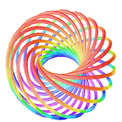
Torus knot of type (15,17).
This chapter shows how to use the FriCAS graphics facilities under the X Window System. FriCAS has two-dimensional and three-dimensional drawing and rendering packages that allow the drawing, coloring, transforming, mapping, clipping, and combining of graphic output from FriCAS computations. This facility is particularly useful for investigating problems in areas such as topology. The graphics package is capable of plotting functions of one or more variables or plotting parametric surfaces and curves. Various coordinate systems are also available, such as polar and spherical.
A graph is displayed in a viewport window and it has a control-panel that uses interactive mouse commands. PostScript and other output forms are available so that FriCAS images can be printed or used by other programs.1
The FriCAS two-dimensional graphics package provides the ability to display
These graphs can be modified by specifying various options, such as calculating points in the polar coordinate system or changing the size of the graph viewport window.
The first kind of two-dimensional graph is that of a curve defined by a function y = f(x) over a finite interval of
the x axis.
The general format for drawing a function defined by a formula f(x) is:
draw(f(x), x = a..b, options)
where a..b defines the range of x, and where options prescribe zero or more options as described in Section
7.1.4 on page 399. An example of an option is curveColor == bright red(). An alternative format involving
functions f and g is also available.
A simple way to plot a function is to use a formula. The first argument is the formula. For the second
argument, write the name of the independent variable (here, x), followed by an “=”, and the range of
values.
Display this formula over the range  . FriCAS converts your formula to a compiled function so that
the results can be computed quickly and efficiently.
draw(sin(tan(x)) - tan(sin(x)),x = 0..6)
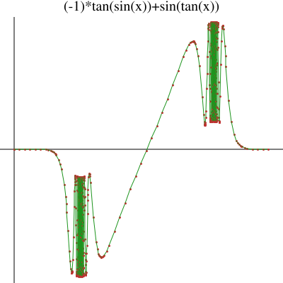
Notice that FriCAS compiled the function before the graph was put on the screen.
Here is the same graph on a different interval. This time we give the graph a title.
draw(sin(tan(x)) - tan(sin(x)), x = 10..16, title=="Shifted view")
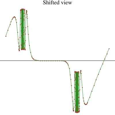
Once again the formula is converted to a compiled function before any points are computed. If you want to graph the same function on several intervals, it is a good idea to define the function first so that the function has to be compiled only once. This time we first define the function.
f(x) == (x-1)*(x-2)*(x-3)
To draw the function, the first argument is its name and the second is just the range with no independent variable.
draw(f, 0..4)
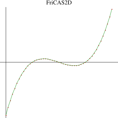
The second kind of two-dimensional graph is that of curves produced by parametric equations. Let x = f(t)
and y = g(t) be formulas or two functions f and g as the parameter t ranges over an interval [a,b]. The
function curve takes the two functions f and g as its parameters.
The general format for drawing a two-dimensional plane curve defined by parametric formulas x = f(t) and
y = g(t) is:
draw(curve(f(t), g(t)), t = a..b, options)
where a..b defines the range of the independent variable t, and where options prescribe zero or more options
as described in Section 7.2.4 on page 438. An example of an option is curveColor == bright red().
Here’s an example:
Define a parametric curve using a range involving %pi, FriCAS’s way of saying  . For parametric curves,
FriCAS compiles two functions, one for each of the functions
f and g.
draw(curve(sin(t)*sin(2*t)*sin(3*t), sin(4*t)*sin(5*t)*sin(6*t)), t = 0..2*%pi)
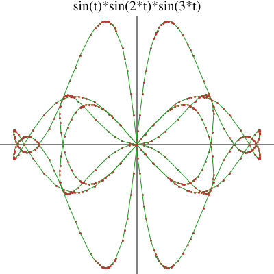
The title may be an arbitrary string and is an optional argument to the draw command.
draw(curve(cos(t), sin(t)), t = 0..2*%pi, title=="Circle")
If you plan on plotting x = f(t), y = g(t) as t ranges over several intervals, you may want to define functions f
and g first, so that they need not be recompiled every time you create a new graph. Here’s an example: As
before, you can first define the functions you wish to draw.
f(t:DFLOAT):DFLOAT == sin(3*t/4)
Function declaration f : DoubleFloat -> DoubleFloat has been added to workspace.
FriCAS compiles them to map DoubleFloat values to DoubleFloat values.
g(t:DFLOAT):DFLOAT == sin(t)
Function declaration g : DoubleFloat -> DoubleFloat has been added to workspace.
Give to curve the names of the functions, then write the range without the name of the independent variable.
draw(curve(f,g),0..%pi)
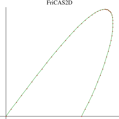
Here is another look at the same curve but over a different range. Notice that f and g are not
recompiled. Also note that FriCAS provides a default title based on the first function specified in
curve.
draw(curve(f,g),-4*%pi..4*%pi)
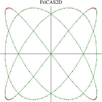
A third kind of two-dimensional graph is a non-singular “solution curve” in a rectangular region of the plane.
A solution curve is a curve defined by a polynomial equation p(x,y)= 0. Non-singular means that the curve is
“smooth” in that it does not cross itself or come to a point (cusp). Algebraically, this means that for any
point (x,y) on the curve, that is, a point such that p(x,y)= 0, the partial derivatives  and
 are not both zero.
The general format for drawing a non-singular solution curve given by a polynomial of the form p(x,y)= 0 is:
draw(p(x,y) = 0, x, y, range == [a..b, c..d], options)
where the second and third arguments name the first and second independent variables of p. A range option
is always given to designate a bounding rectangular region of the plane  . Zero or more
additional options as described in Section 7.1.4 on page 399 may be given.
We require that the polynomial has rational or integral coefficients. Here is an algebraic curve example (“Cartesian ovals”):
p := ((x^2 + y^2 + 1) - 8*x)^2 - (8*(x^2 + y^2 + 1)-4*x-1)
The first argument is always expressed as an equation of the form p = 0 where p is a polynomial.
draw(p = 0, x, y, range == [-1..11, -7..7])
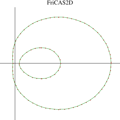
The draw commands take an optional list of options, such as title shown above. Each option is given by the syntax: name == value. Here is a list of the available options in the order that they are described below.
| adaptive | clip | unit |
| clip | curveColor | range |
| toScale | pointColor | coordinates |
The adaptive option turns adaptive plotting on or off. Adaptive plotting uses an algorithm that traverses a
graph and computes more points for those parts of the graph with high curvature. The higher the curvature of
a region is, the more points the algorithm computes. The adaptive option is normally on. Here we turn it
off.
draw(sin(1/x),x=-2*%pi..2*%pi, adaptive == false)
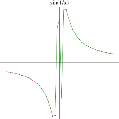
The clip option turns clipping on or off. If on, large values are cut off according to clipPointsDefault.
draw(tan(x),x=-2*%pi..2*%pi, clip == true)
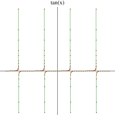
Option toScale does plotting to scale if true or uses the entire viewport if false. The default can be determined using drawToScale.
draw(sin(x),x=-%pi..%pi, toScale == true, unit == [1.0,1.0])
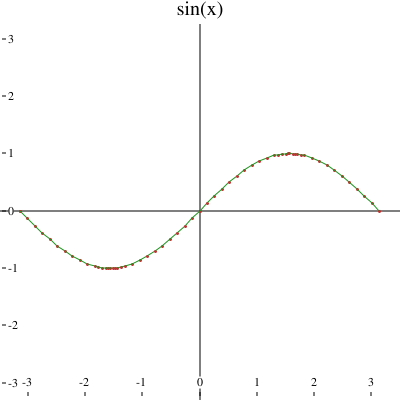
Option clip with a range sets point clipping of a graph within the ranges specified in the list
[x range, y range]. If only one range is specified, clipping applies to the y-axis.
draw(sec(x),x=-2*%pi..2*%pi, clip == [-2*%pi..2*%pi,-%pi..%pi], unit == [1.0,1.0])
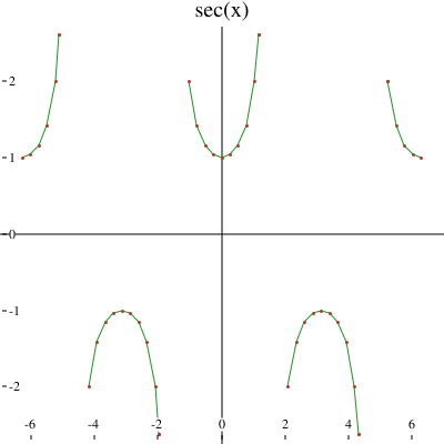
Option curveColor sets the color of the graph curves or lines to be the indicated palette color (see Section 7.1.5 on page 402 and Section 7.1.6 on page 403).
draw(sin(x),x=-%pi..%pi, curveColor == bright red())
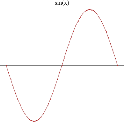
Option pointColor sets the color of the graph points to the indicated palette color (see Section 7.1.5 on page 402 and Section 7.1.6 on page 403).
draw(sin(x),x=-%pi..%pi, pointColor == pastel yellow())
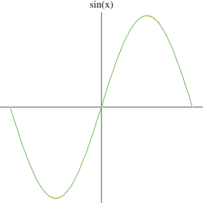
Option unit sets the intervals at which the axis units are plotted according to the indicated steps [x interval,
y interval].
draw(curve(9*sin(3*t/4),8*sin(t)), t = -4*%pi..4*%pi, unit == [2.0,1.0])
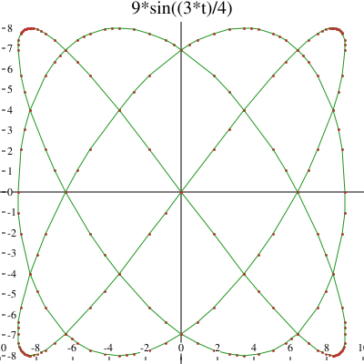
Option range sets the range of variables in a graph to be within the ranges for solving plane algebraic curve plots.
draw(y^2 + y - (x^3 - x) = 0, x, y, range == [-2..2,-2..1], unit==[1.0,1.0])
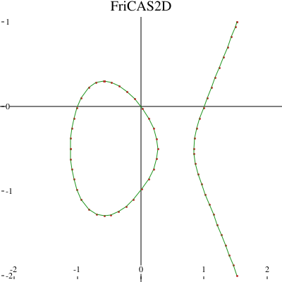
A second example of a solution plot.
draw(x^2 + y^2 = 1, x, y, range == [-3/2..3/2,-3/2..3/2], unit==[0.5,0.5])
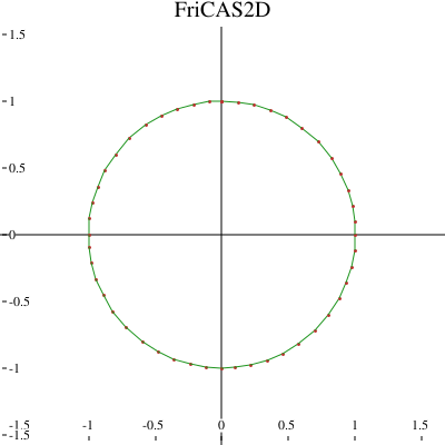
Option coordinates indicates the coordinate system in which the graph is plotted. The default is to use the
Cartesian coordinate system. For more details, see Section 7.2.7 on page 455.
draw(curve(sin(5*t),t),t=0..2*%pi, coordinates == polar)
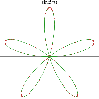
The domain Color provides operations for manipulating colors in two-dimensional graphs. Colors
are objects of Color. Each color has a hue and a weight. Hues are represented by integers that
range from 1 to the numberOfHues(), normally 27. Weights are floats and have the value 1.0 by
default.
(integer)
creates a color of hue integer and weight 1.0.
(), blue() green(), and yellow()
create colors of that hue with weight 1.0.
 +

returns the color that results from additively combining the indicated  and
 . Color
addition is not commutative: changing the order of the arguments produces different results.
changes the weight of color by integer without affecting its hue. For example, red()+ 3*yellow()
produces a color closer to yellow than to red. Color multiplication is not associative: changing
the order of grouping produces different results.
These functions can be used to change the point and curve colors for two- and three-dimensional graphs. Use the pointColor option for points.
draw(x^2,x=-1..1,pointColor == green())
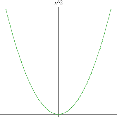
Use the curveColor option for curves.
draw(x^2,x=-1..1,curveColor == color(13) + 2*blue())
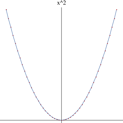
Domain Palette is the domain of shades of colors: dark, dim, bright, pastel, and light, designated by the
integers 1 through 5, respectively. Colors are normally “bright.”
shade red()
PositiveInteger To change the shade of a color, apply the name of a shade to it.
myFavoriteColor := dark blue()
Palette The expression shade(color) returns the value of a shade of color.
shade myFavoriteColor
PositiveInteger The expression hue(color) returns its hue.
hue myFavoriteColor
Color Palettes can be used in specifying colors in two-dimensional graphs.
draw(x^2,x=-1..1,curveColor == dark blue())
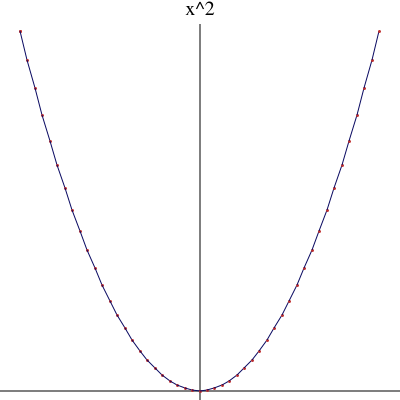
Once you have created a viewport, move your mouse to the viewport and click with your left mouse button to display a control-panel. The panel is displayed on the side of the viewport closest to where you clicked. Each of the buttons which toggle on and off show the current state of the graph.
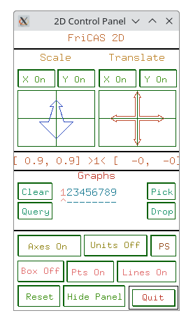
Two-dimensional control-panel.
Object transformations are executed from the control-panel by mouse-activated potentiometer windows.
To scale a graph, click on a mouse button within the Scale window in the upper left corner of the control-panel. The axes along which the scaling is to occur are indicated by setting the toggles above the arrow. With X On and Y On appearing, both axes are selected and scaling is uniform. If either is not selected, for example, if X Off appears, scaling is non-uniform.
To translate a graph, click the mouse in the Translate window in the direction you wish the graph to move. This window is located in the upper right corner of the control-panel. Along the top of the Translate window are two buttons for selecting the direction of translation. Translation along both coordinate axes results when X On and Y On appear or along one axis when one is on, for example, X On and Y Off appear.
The window directly below the transformation potentiometer windows is used to display system messages
relating to the viewport and the control-panel. The following format is displayed:
[scaleX, scaleY] >graph< [translateX, translateY]
The two values to the left show the scale factor along the X and Y coordinate axes. The two values to the right show the distance of translation from the center in the X and Y directions. The number in the center shows which graph in the viewport this data pertains to. When multiple graphs exist in the same viewport, the graph must be selected (see “Multiple Graphs,” below) in order for its transformation data to be shown, otherwise the number is 1.
The Graphs window contains buttons that allow the placement of two-dimensional graphs into one of nine available slots in any other two-dimensional viewport. In the center of the window are numeral buttons from one to nine that show whether a graph is displayed in the viewport. Below each number button is a button showing whether a graph that is present is selected for application of some transformation. When the caret symbol is displayed, then the graph in that slot will be manipulated. Initially, the graph for which the viewport is created occupies the first slot, is displayed, and is selected.
The Clear button deselects every viewport graph slot. A graph slot is reselected by selecting the button below its number.
The Query button is used to display the scale and translate data for the indicated graph. When this button is selected the message “Click on the graph to query” appears. Select a slot number button from the Graphs window. The scaling factor and translation offset of the graph are then displayed in the message window.
The Pick button is used to select a graph to be placed or dropped into the indicated viewport. When this button is selected, the message “Click on the graph to pick” appears. Click on the slot with the graph number of the desired graph. The graph information is held waiting for you to execute a Drop in some other graph.
Once a graph has been picked up using the Pick button, the Drop button places it into a new viewport slot. The message “Click on the graph to drop” appears in the message window when the Drop button is selected. By selecting one of the slot number buttons in the Graphs window, the graph currently being held is dropped into this slot and displayed.
encloses the area of the viewport graph in a bounding box, or removes the box if already enclosed.
writes the current viewport contents to a file fricas2D.ps. The file is placed in the directory from which FriCAS or the viewAlone program was invoked.
resets the object transformation characteristics and attributes back to their initial states.
queries whether the current viewport session should be terminated.
Here is a summary of useful FriCAS operations for two-dimensional graphics. Each operation name is followed by a list of arguments. Each argument is written as a variable informally named according to the type of the argument (for example, integer). If appropriate, a default value for an argument is given in parentheses immediately following the name.
([boolean(true)])
sets or indicates whether graphs are plotted according to the adaptive refinement algorithm.
([color(dark blue())])
sets or indicates the default color of the axes in a two-dimensional graph viewport.
([boolean(false)])
sets or indicates whether point clipping is to be applied as the default for graph plots.
([boolean(false)])
sets or indicates whether the plot of a graph is “to scale” or uses the entire viewport space as
the default.
([color(pastel yellow())])
sets or indicates the default color of the lines or curves in a two-dimensional graph viewport.
([integer(500)])
sets or indicates the default maximum number of possible points to be used when constructing
a two-dimensional graph.
([integer(21)])
sets or indicates the default minimum number of possible points to be used when constructing
a two-dimensional graph.
([color(bright red())])
sets or indicates the default color of the points in a two-dimensional graph viewport.
([integer(5)])
sets or indicates the default size of the dot used to plot points in a two-dimensional graph.
([integer(600)])
sets or indicates the default screen resolution constant used in setting the computation limit of
adaptively generated curve plots.
([color(dim green())])
sets or indicates the default color of the unit labels in a two-dimensional graph viewport.
()
resets the default settings for the following attributes: point color, line color, axes color, units
color, point size, viewport upper left-hand corner position, and the viewport size.
([list([100,100])])
sets or indicates the default position of the upper left-hand corner of a two-dimensional viewport,
relative to the display root window. The upper left-hand corner of the display is considered to
be at the (0, 0) position.
([list([200,200])])
sets or indicates the default size in which two dimensional viewport windows are shown. It is
defined by a width and then a height.
([list(["pixmap", "bitmap", "postscript", "image")])
indicates the possible file types that can be created with the ‘write‘ function.
([list([])])
sets or indicates the default types of files, in addition to the data file, that are created when a
write function is executed on a viewport.
(viewport, integer(1), string("off"))
turns the units on or off for the graph with index integer.
(viewport, integer(1), string("on"))
turns the axes on or off for the graph with index integer.
(viewport, integer(1), string("on"))
declares whether lines connecting the points are displayed or not.
(viewport, string("off"))
declares whether the two-dimensional control-panel is automatically displayed or not.
(viewport)
returns a list describing the state of each graph. If the graph state is not being used this is shown
by "undefined", otherwise a description of the graph’s contents is shown.
(viewport)
displays a list of all the graph states available for viewport, giving the values for every property.
(viewport,  (viewPosDefault),
 (viewPosDefault))
moves viewport on the screen so that the upper left-hand corner of viewport is at the position
(x,y).
(viewport)
returns a list of all the DrawOptions used by viewport.
(viewport, integer(1), string("on"))
specifies whether the graph points for graph integer are to be displayed or not.
(viewport, integer(1), string("off"))
declares whether graph integer is or is not to be displayed with a bounding rectangle.
(viewport)
resets all the properties of viewport.
(viewport,  ,
 )
resizes viewport with a new width and height.
(viewport,  (1),
 (0.9),
 (0.9))
scales values for the x and y coordinates of graph n.
(viewport,  (1), string("on"))
indicates if graph n is shown or not.
(viewport, string("FriCAS 2D"))
designates the title for viewport.
(viewport,  (1),
 (0.0),
 (0.0))
causes graph n to be moved x and y units in the respective directions.
(viewport,  , [strings])
if no third argument is given, writes the data file into the directory with extension data. The
third argument can be a single string or a list of strings with some or all the entries "pixmap",
"bitmap", "postscript", and "image".
In this section we demonstrate how to create two-dimensional graphs from lists of points and give an example showing how to read the lists of points from a file.
FriCAS creates lists of points in a two-dimensional viewport by utilizing the GraphImage and TwoDimensionalViewport domains. In this example, the makeGraphImage function takes a list of lists of points as a parameter, a list of colors for each point in the graph, a list of colors for each line in the graph, and a list of sizes for each point in the graph. The following expressions create a list of lists of points which will be read by FriCAS and made into a two-dimensional viewport.
p1 := point [1,1]$(Point DFLOAT)
p2 := point [0,1]$(Point DFLOAT)
p3 := point [0,0]$(Point DFLOAT)
p4 := point [1,0]$(Point DFLOAT)
p5 := point [1,.5]$(Point DFLOAT)
p6 := point [.5,0]$(Point DFLOAT)
p7 := point [0,0.5]$(Point DFLOAT)
p8 := point [.5,1]$(Point DFLOAT)
p9 := point [.25,.25]$(Point DFLOAT)
p10 := point [.25,.75]$(Point DFLOAT)
p11 := point [.75,.75]$(Point DFLOAT)
p12 := point [.75,.25]$(Point DFLOAT)
Point(DoubleFloat) Finally, here is the list.
llp := [[p1,p2], [p2,p3], [p3,p4], [p4,p1], [p5,p6], [p6,p7], [p7,p8], [p8,p5], [p9,p10], [p10,p11], [p11,p12], [p12,p9]]
List(List(Point(DoubleFloat))) Now we set the point sizes for all components of the graph.
size1 := 6::PositiveInteger
size2 := 8::PositiveInteger
size3 := 10::PositiveInteger
lsize := [size1, size1, size1, size1, size2, size2, size2, size2, size3, size3, size3, size3]
List(PositiveInteger) Here are the colors for the points.
pc1 := pastel red()
pc2 := dim green()
pc3 := pastel yellow()
lpc := [pc1, pc1, pc1, pc1, pc2, pc2, pc2, pc2, pc3, pc3, pc3, pc3]
List(Palette) Here are the colors for the lines.
lc := [pastel blue(), light yellow(), dim green(), bright red(), light green(), dim yellow(), bright blue(), dark red(), pastel red(), light blue(), dim green(), light yellow()]
List(Palette) Now the GraphImage is created according to the component specifications indicated above.
g := makeGraphImage(llp,lpc,lc,lsize)$GRIMAGE
GraphImage The makeViewport2D function now creates a TwoDimensionalViewport for this graph according to the list of options specified within the brackets.
makeViewport2D(g,[title("Lines")])$VIEW2D
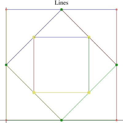
This example demonstrates the use of the GraphImage functions component and appendPoint in adding points to an empty GraphImage.
)clear all
All user variables and function definitions have been cleared.
g := graphImage()$GRIMAGE
p1 := point [0,0]$(Point DFLOAT)
p2 := point [.25,.25]$(Point DFLOAT)
p3 := point [.5,.5]$(Point DFLOAT)
p4 := point [.75,.75]$(Point DFLOAT)
p5 := point [1,1]$(Point DFLOAT)
component(g,p1)$GRIMAGE
component(g,p2)$GRIMAGE
appendPoint(g,p3)$GRIMAGE
appendPoint(g,p4)$GRIMAGE
appendPoint(g,p5)$GRIMAGE
Here is the graph.
makeViewport2D(g,[title("Graph Points")])$VIEW2D
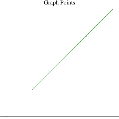
A list of points can also be made into a GraphImage by using the operation coerce. It is equivalent to
adding each point to g2 using component.
g2 := coerce([[p1],[p2],[p3],[p4],[p5]])$GRIMAGE
GraphImage Now, create an empty TwoDimensionalViewport.
v := viewport2D()$VIEW2D
options(v,[title("Just Points")])$VIEW2D
TwoDimensionalViewport Place the graph into the viewport.
putGraph(v,g2,1)$VIEW2D
Take a look.
makeViewport2D(v)$VIEW2D
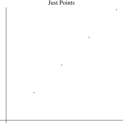
The following three functions read a list of points from a file and then draw the points and the connecting
lines. The points are stored in the file in readable form as floating point numbers (specifically, DoubleFloat
values) as an alternating stream of x- and y-values. For example,
0.0 0.0 1.0 1.0 2.0 4.0 3.0 9.0 4.0 16.0 5.0 25.0
1drawPoints(lp:List Point DoubleFloat):VIEW2D == 2 g := graphImage()$GRIMAGE 3 for p in lp repeat 4 component(g,p,pointColorDefault(),lineColorDefault(), 5 pointSizeDefault()) 6 makeViewport2D(g,[title("Points")])$VIEW2D 7 8drawLines(lp:List Point DoubleFloat):VIEW2D == 9 g := graphImage()$GRIMAGE 10 component(g, lp, pointColorDefault(), lineColorDefault(), 11 pointSizeDefault())$GRIMAGE 12 makeViewport2D(g,[title("Points")])$VIEW2D 13 14plotData2D(name, title) == 15 f:File(DFLOAT) := open(name,"input") 16 lp:LIST(Point DFLOAT) := empty() 17 while ((x := readIfCan!(f)) case DFLOAT) repeat 18 y : DFLOAT := read!(f) 19 lp := cons(point [x,y]$(Point DFLOAT), lp) 20 lp 21 close!(f) 22 drawPoints(lp) 23 drawLines(lp) 24
This command will actually create the viewport and the graph if the point data is in the file
"file.data".
1plotData2D("file.data", "2D Data Plot") 2
This section demonstrates how to append a two-dimensional graph to a viewport already containing other graphs. The default draw command places a graph into the first GraphImage slot position of the TwoDimensionalViewport.
This graph is in the first slot in its viewport.
v1 := draw(sin(x),x=0..2*%pi)
Compiling function %C with type DoubleFloat -> DoubleFloat
TwoDimensionalViewport So is this graph.
v2 := draw(cos(x),x=0..2*%pi, curveColor==light red())
Compiling function %E with type DoubleFloat -> DoubleFloat
TwoDimensionalViewport The operation getGraph retrieves the GraphImage g1 from the first slot position in the viewport
v1.
g1 := getGraph(v1,1)
GraphImage Now putGraph places g1 into the second slot position of v2.
putGraph(v2,g1,2)
Display the new TwoDimensionalViewport containing both graphs.
makeViewport2D(v2)
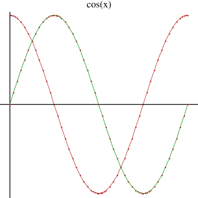
Instead of using draw to draw a graph and then extract graph data we can use makeObject. First graph.
g3 := makeObject(sin(x),x=-1..%pi,[])
Compiling function %G with type DoubleFloat -> DoubleFloat
GraphImage This graph is in the first slot in its viewport.
v3 := draw(cos(x),x=-1..%pi, curveColor==light red())
Compiling function %I with type DoubleFloat -> DoubleFloat
TwoDimensionalViewport Now putGraph places g3 into the second slot position of v3.
putGraph(v3,g3,2)
Display the new TwoDimensionalViewport containing both graphs.
makeViewport2D(v3)
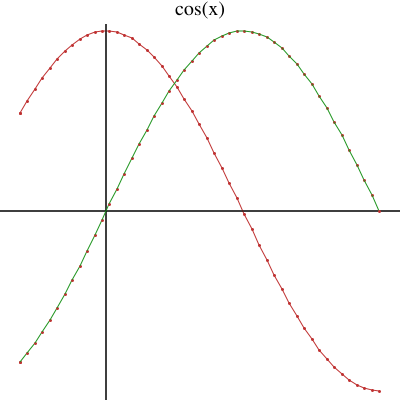
The viewports v1, v2 and v3 are no longer needed so we close them.
close(v1); close(v2); close(v3)
The FriCAS three-dimensional graphics package provides the ability to
These graphs can be modified by using various options, such as calculating points in the spherical coordinate system or changing the polygon grid size of a surface.
The simplest three-dimensional graph is that of a surface defined by a function of two variables,
z = f(x,y).
The general format for drawing a surface defined by a formula f(x,y) of two variables x and y is:
draw(f(x,y), x = a..b, y = c..d, options)
where a..b and c..d define the range of x and y, and where options prescribe zero or more options as
described in Section 7.2.4 on page 438. An example of an option is title == "Title of Graph". An alternative
format involving a function f is also available.
The simplest way to plot a function of two variables is to use a formula. With formulas you always precede the range specifications with the variable name and an “=” sign. Notice that FriCAS uses the text of your function as a default title.
draw(cos(x*y),x=-3..3,y=-3..3)
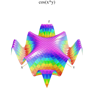
If you intend to use a function more than once, or it is long and complex, then first give its definition to FriCAS.
f(x,y) == sin(x)*cos(y)
To draw the function, just give its name and drop the variables from the range specifications. FriCAS compiles your function for efficient computation of data for the graph.
draw(f,-%pi..%pi,-%pi..%pi)
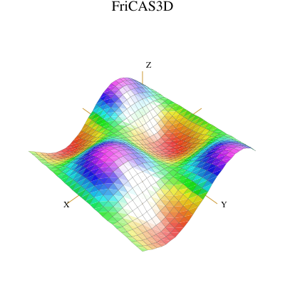
A second kind of three-dimensional graph is a three-dimensional space curve defined by the parametric
equations for x(t), y(t), and z(t) as a function of an independent variable t.
The general format for drawing a three-dimensional space curve defined by parametric formulas x = f(t),
y = g(t), and z = h(t) is:
draw(curve(f(t),g(t),h(t)), t = a..b, options)
where a..b defines the range of the independent variable t, and where options prescribe zero or more options
as described in Section 7.2.4 on page 438. An example of an option is title == "Title of Graph". An
alternative format involving functions f, g and h is also available.
If you use explicit formulas to draw a space curve, always precede the range specification with the variable name and an “=” sign.
draw(curve(5*cos(t), 5*sin(t),t), t=-12..12)
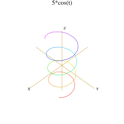
Alternatively, you can draw space curves by referring to functions.
i1(t:DFLOAT):DFLOAT == sin(t)*cos(3*t/5)
Function declaration i1 : DoubleFloat -> DoubleFloat has been added to workspace.
This is useful if the functions are to be used more than once …
i2(t:DFLOAT):DFLOAT == cos(t)*cos(3*t/5)
Function declaration i2 : DoubleFloat -> DoubleFloat has been added to workspace.
or if the functions are long and complex.
i3(t:DFLOAT):DFLOAT == cos(t)*sin(3*t/5)
Function declaration i3 : DoubleFloat -> DoubleFloat has been added to workspace.
Give the names of the functions and drop the variable name specification in the second argument. Again, FriCAS supplies a default title.
draw(curve(i1,i2,i3),0..15*%pi)
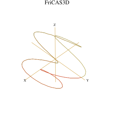
A third kind of three-dimensional graph is a surface defined by parametric equations for x(u,v), y(u,v), and
z(u,v) of two independent variables u and v.
The general format for drawing a three-dimensional graph defined by parametric formulas x = f(u,v),
y = g(u,v), and z = h(u,v) is:
draw(surface(f(u,v),g(u,v),h(u,v)), u = a..b, v = c..d, options)
where a..b and c..d define the range of the independent variables u and v, and where options
prescribe zero or more options as described in Section 7.2.4 on page 438. An example of an option is
title == "Title of Graph". An alternative format involving functions f, g and h is also available.
This example draws a graph of a surface plotted using the parabolic cylindrical coordinate system option. The values of the functions supplied to surface are interpreted in coordinates as given by a coordinates option, here as parabolic cylindrical coordinates (see Section 7.2.7 on page 455).
draw(surface(u*cos(v), u*sin(v), v*cos(u)), u=-4..4, v=0..%pi, coordinates== parabolicCylindrical)
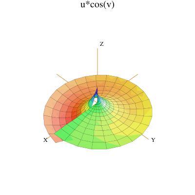
Again, you can graph these parametric surfaces using functions, if the functions are long and complex. Here we declare the types of arguments and values to be of type DoubleFloat.
n1(u:DFLOAT,v:DFLOAT):DFLOAT == u*cos(v)
Function declaration n1 : (DoubleFloat, DoubleFloat) -> DoubleFloat has been added to workspace.
As shown by previous examples, these declarations are necessary.
n2(u:DFLOAT,v:DFLOAT):DFLOAT == u*sin(v)
Function declaration n2 : (DoubleFloat, DoubleFloat) -> DoubleFloat has been added to workspace.
In either case, FriCAS compiles the functions when needed to graph a result.
n3(u:DFLOAT,v:DFLOAT):DFLOAT == u
Function declaration n3 : (DoubleFloat, DoubleFloat) -> DoubleFloat has been added to workspace.
Without these declarations, you have to suffix floats with @DFLOAT to get a DoubleFloat result. However, a
call here with an unadorned float produces a DoubleFloat.
n3(0.5,1.0)
Compiling function n3 with type (DoubleFloat, DoubleFloat) -> DoubleFloat
DoubleFloat Draw the surface by referencing the function names, this time choosing the toroidal coordinate system.
draw(surface(n1,n2,n3), 1..4, 1..2*%pi, coordinates == toroidal(1$DFLOAT))
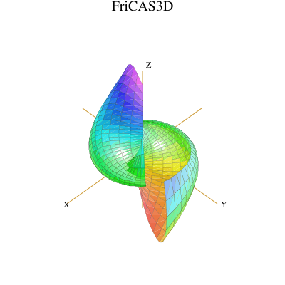
The draw commands optionally take an optional list of options such as coordinates as shown in the last
example. Each option is given by the syntax: name == value. Here is a list of the available options in the order
that they are described below:
| title | coordinates | var1Steps |
| style | tubeRadius | var2Steps |
| colorFunction | tubePoints | space |
The option title gives your graph a title.
draw(cos(x*y),x=0..2*%pi,y=0..%pi,title == "Title of Graph")
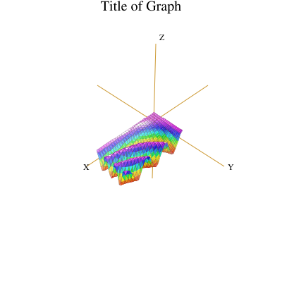
The style determines which of four rendering algorithms is used for the graph. The choices are "wireMesh",
"solid", "shade", and "smooth".
draw(cos(x*y),x=-3..3,y=-3..3, style=="smooth", title=="Smooth Option")
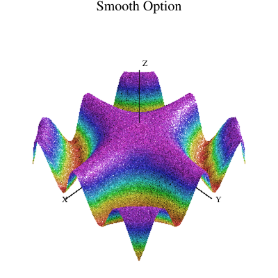
In all but the wire-mesh style, polygons in a surface or tube plot are normally colored in a graph according to
their z-coordinate value. Space curves are colored according to their parametric variable value. To change this,
you can give a coloring function. The coloring function is sampled across the range of its arguments, then
normalized onto the standard FriCAS colormap.
A function of one variable makes the color depend on the value of the parametric variable specified for a tube plot.
color1(t) == t
draw(curve(sin(t), cos(t),0), t=0..2*%pi, tubeRadius == .3, colorFunction == color1)
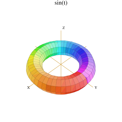
A function of two variables makes the color depend on the values of the independent variables.
color2(u,v) == u^2 - v^2
Use the option colorFunction for special coloring.
draw(cos(u*v), u=-3..3, v=-3..3, colorFunction == color2)
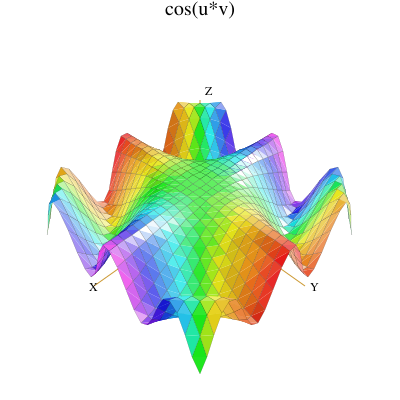
With a three variable function, the color also depends on the value of the function.
color3(x,y,fxy) == sin(x*fxy) + cos(y*fxy)
draw(cos(x*y), x=-3..3, y=-3..3, colorFunction == color3)
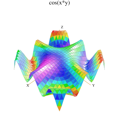
Normally the Cartesian coordinate system is used. To change this, use the coordinates option. For details, see Section 7.2.7 on page 455.
m(u:DFLOAT,v:DFLOAT):DFLOAT == 1
Function declaration m : (DoubleFloat, DoubleFloat) -> DoubleFloat has been added to workspace.
Use the spherical coordinate system.
draw(m, 0..2*%pi,0..%pi, coordinates == spherical, style=="shade")
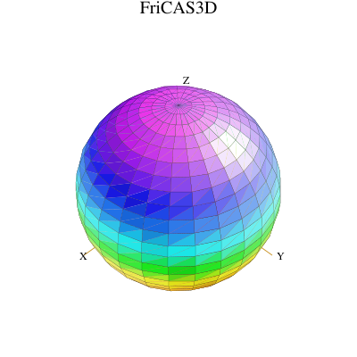
Space curves may be displayed as tubes with polygonal cross sections. Two options, tubeRadius and tubePoints, control the size and shape of this cross section. The tubeRadius option specifies the radius of the tube that encircles the specified space curve.
draw(curve(sin(t),cos(t),0),t=0..2*%pi, style=="shade", tubeRadius == .3)
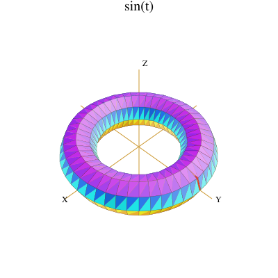
The tubePoints option specifies the number of vertices defining the polygon that is used to create a tube around the specified space curve. The larger this number is, the more cylindrical the tube becomes.
draw(curve(sin(t), cos(t), 0), t=0..2*%pi, style=="shade", tubeRadius == .25, tubePoints == 3)
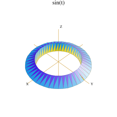
Options var1Steps and var2Steps specify the number of intervals into which the grid defining a surface plot is subdivided with respect to the first and second parameters of the surface function(s).
draw(cos(x*y),x=-3..3,y=-3..3, style=="shade", var1Steps == 30, var2Steps == 30)
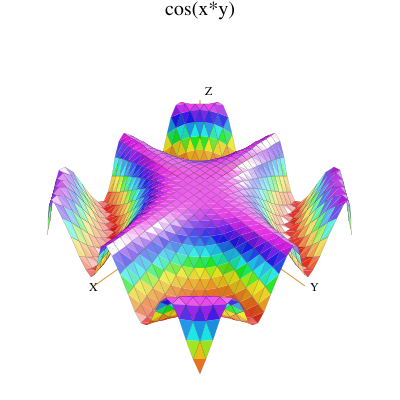
The space option of a draw command lets you build multiple graphs in three space. To use this option, first create an empty three-space object, then use the space option thereafter. There is no restriction as to the number or kinds of graphs that can be combined this way. Create an empty three-space object.
s := create3Space()$(ThreeSpace DFLOAT)
m(u:DFLOAT,v:DFLOAT):DFLOAT == 1
Function declaration m : (DoubleFloat, DoubleFloat) -> DoubleFloat has been added to workspace.
1 old definition(s) deleted for function or rule m
Add a graph to this three-space object. The new graph destructively inserts the graph into s.
draw(m,0..%pi,0..2*%pi, coordinates == spherical, space == s)
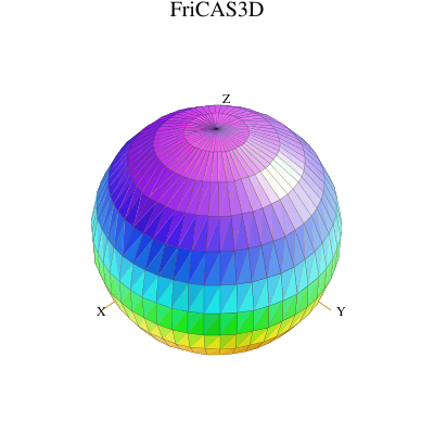
Add a second graph to s.
v := draw(curve(1.5*sin(t), 1.5*cos(t),0), t=0..2*%pi, tubeRadius == .25, space == s)
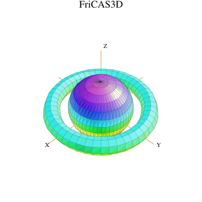
A three-space object can also be obtained from an existing three-dimensional viewport using the subspace
command. You can then use makeViewport3D to create a viewport window. Assign to subsp the three-space
object in viewport v.
subsp := subspace v
Reset the space component of v to the value of subsp.
subspace(v, subsp)
Create a viewport window from a three-space object.
makeViewport3D(subsp,"Graphs")
An alternate way to create multiple graphs is to use makeObject. The makeObject command is similar to the draw command, except that it returns a three-space object rather than a ThreeDimensionalViewport. In fact, makeObject is called by the draw command to create the ThreeSpace then makeViewport3D to create a viewport window.
m(u:DFLOAT,v:DFLOAT):DFLOAT == 1
Function declaration m : (DoubleFloat, DoubleFloat) -> DoubleFloat has been added to workspace.
Do the last example a new way. First use makeObject to create a three-space object sph.
sph := makeObject(m, 0..%pi, 0..2*%pi, coordinates==spherical)
Compiling function m with type (DoubleFloat, DoubleFloat) -> DoubleFloat
ThreeSpace(DoubleFloat) Add a second object to sph.
makeObject(curve(1.5*sin(t), 1.5*cos(t), 0), t=0..2*%pi, space == sph, tubeRadius == .25)
Compiling function %M with type DoubleFloat -> DoubleFloat
Compiling function %O with type DoubleFloat -> DoubleFloat
Compiling function %Q with type DoubleFloat -> DoubleFloat
ThreeSpace(DoubleFloat) Create and display a viewport containing sph.
makeViewport3D(sph,"Multiple Objects")
Note that an undefined ThreeSpace parameter declared in a makeObject or draw command results in an error. Use the create3Space function to define a ThreeSpace, or obtain a ThreeSpace that has been previously generated before including it in a command line.
Rather than using the draw and makeObject commands, you can create three-dimensional graphs from primitives. Operation create3Space creates a three-space object to which points, curves and polygons can be added using the operations from the ThreeSpace domain. The resulting object can then be displayed in a viewport using makeViewport3D.
Create the empty three-space object space.
space := create3Space()$(ThreeSpace DFLOAT)
Objects can be sent to this space using the operations exported by the ThreeSpace domain. The following
examples place curves into space.
Add these eight curves to the space.
closedCurve(space,[[0,30,20], [0,30,30], [0,40,30], [0,40,100], [0,30,100],[0,30,110], [0,60,110], [0,60,100], [0,50,100], [0,50,30], [0,60,30], [0,60,20]])
closedCurve(space,[[80,0,30], [80,0,100], [70,0,110], [40,0,110], [30,0,100], [30,0,90], [40,0,90], [40,0,95], [45,0,100], [65,0,100], [70,0,95], [70,0,35]])
closedCurve(space,[[70,0,35], [65,0,30], [45,0,30], [40,0,35], [40,0,60], [50,0,60], [50,0,70], [30,0,70], [30,0,30], [40,0,20], [70,0,20], [80,0,30]])
closedCurve(space,[[0,70,20], [0,70,110], [0,110,110], [0,120,100], [0,120,70], [0,115,65], [0,120,60], [0,120,30], [0,110,20], [0,80,20], [0,80,30], [0,80,20]])
closedCurve(space,[[0,105,30], [0,110,35], [0,110,55], [0,105,60], [0,80,60], [0,80,70], [0,105,70], [0,110,75], [0,110,95], [0,105,100], [0,80,100], [0,80,20], [0,80,30]])
closedCurve(space,[[140,0,20], [140,0,110], [130,0,110], [90,0,20], [101,0,20],[114,0,50], [130,0,50], [130,0,60], [119,0,60], [130,0,85], [130,0,20]])
closedCurve(space,[[0,140,20], [0,140,110], [0,150,110], [0,170,50], [0,190,110], [0,200,110], [0,200,20], [0,190,20], [0,190,75], [0,175,35], [0,165,35],[0,150,75], [0,150,20]])
closedCurve(space,[[200,0,20], [200,0,110], [189,0,110], [160,0,45], [160,0,110], [150,0,110], [150,0,20], [161,0,20], [190,0,85], [190,0,20]])
ThreeSpace(DoubleFloat) Create and display the viewport using makeViewport3D. Options may also be given but here are displayed as a list with values enclosed in parentheses.
makeViewport3D(space, title == "Letters")
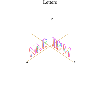
As a second example of the use of primitives, we generate a cube using a polygon mesh. It is important to use a consistent orientation of the polygons for correct generation of three-dimensional objects.
Again start with an empty three-space object.
spaceC := create3Space()$(ThreeSpace DFLOAT)
ThreeSpace(DoubleFloat) For convenience, give DoubleFloat values +1 and -1 names.
x: DFLOAT := 1
y: DFLOAT := -1
DoubleFloat Define the vertices of the cube.
a := point [x,x,y,1::DFLOAT]$(Point DFLOAT)
b := point [y,x,y,4::DFLOAT]$(Point DFLOAT)
c := point [y,x,x,8::DFLOAT]$(Point DFLOAT)
d := point [x,x,x,12::DFLOAT]$(Point DFLOAT)
e := point [x,y,y,16::DFLOAT]$(Point DFLOAT)
f := point [y,y,y,20::DFLOAT]$(Point DFLOAT)
g := point [y,y,x,24::DFLOAT]$(Point DFLOAT)
h := point [x,y,x,27::DFLOAT]$(Point DFLOAT)
Point(DoubleFloat) Add the faces of the cube as polygons to the space using a consistent orientation.
polygon(spaceC,[d,c,g,h])
polygon(spaceC,[d,h,e,a])
polygon(spaceC,[c,d,a,b])
polygon(spaceC,[g,c,b,f])
polygon(spaceC,[h,g,f,e])
polygon(spaceC,[e,f,b,a])
ThreeSpace(DoubleFloat) Create and display the viewport.
makeViewport3D(spaceC, title == "Cube")
The CoordinateSystems package provides coordinate transformation functions that map a given data point
from the coordinate system specified into the Cartesian coordinate system. The default coordinate system,
given a triplet (f(u,v), u, v), assumes that z = f(u, v), x = u and y = v, that is, reads the coordinates in (z, x, y)
order.
m(u:DFLOAT,v:DFLOAT):DFLOAT == u^2
Function declaration m : (DoubleFloat, DoubleFloat) -> DoubleFloat has been added to workspace.
Graph plotted in default coordinate system.
draw(m,0..3,0..5)
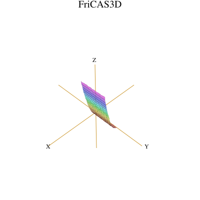
The z coordinate comes first since the first argument of the draw command gives its values. In
general, the coordinate systems FriCAS provides, or any that you make up, must provide a map
to an (x, y, z) triplet in order to be compatible with the coordinates DrawOption. Here is an
example.
Define the identity function.
cartesian(point:Point DFLOAT):Point DFLOAT == point
Function declaration cartesian : Point(DoubleFloat) -> Point(DoubleFloat) has been added to workspace.
Pass cartesian as the coordinates parameter to the draw command.
draw(m,0..3,0..5,coordinates==cartesian)
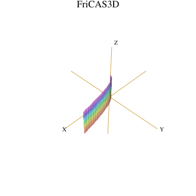
What happened? The option coordinates == cartesian directs FriCAS to treat the dependent variable m
defined by  as the
x coordinate. Thus the triplet of values (m, u, v) is transformed to coordinates
(x, y, z) and so we get the graph of  .
Here is another example. The cylindrical transform takes input of the form (w,u,v), interprets it in the order
( ,
 ,
 ) and maps it to the Cartesian coordinates
 ,
 ,
 in which
 is the
radius,
 is the angle and
 is the z-coordinate. An example using the cylindrical coordinates for the
constant
r = 3.
f(u:DFLOAT,v:DFLOAT):DFLOAT == 3
Function declaration f : (DoubleFloat, DoubleFloat) -> DoubleFloat has been added to workspace.
Graph plotted in cylindrical coordinates.
draw(f,0..%pi,0..6,coordinates==cylindrical)
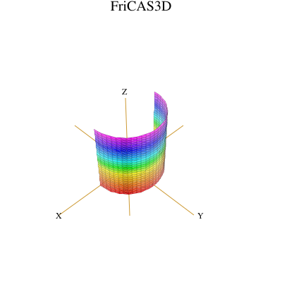
Suppose you would like to specify  as a function of
 and
 instead of just
 ? Well, you still can use
the cylindrical FriCAS transformation but we have to reorder the triplet before passing it to the
transformation.
First, let’s create a point to work with and call it pt with some color col.
col := 5
pt := point[1,2,3,col]$(Point DFLOAT)
Point(DoubleFloat) The reordering you want is  to
 so that the first element is moved to the third
element, while the second and third elements move forward and the color element does not change. Define a
function reorder to reorder the point elements.
reorder(p:Point DFLOAT):Point DFLOAT == point[p.2, p.3, p.1, p.4]
Function declaration reorder : Point(DoubleFloat) -> Point(DoubleFloat) has been added to workspace.
The function moves the second and third elements forward but the color does not change.
reorder pt
Compiling function reorder with type Point(DoubleFloat) -> Point(DoubleFloat)
Point(DoubleFloat) The function newmap converts our reordered version of the cylindrical coordinate system to
the standard  Cartesian system.
newmap(pt:Point DFLOAT):Point DFLOAT == cylindrical(reorder pt)
Function declaration newmap : Point(DoubleFloat) -> Point(DoubleFloat) has been added to workspace.
newmap pt
Compiling function newmap with type Point(DoubleFloat) -> Point(DoubleFloat)
Point(DoubleFloat) Graph the same function f using the coordinate mapping of the function newmap, so it is now
interpreted as  :
draw(f,0..3,0..2*%pi,coordinates==newmap)
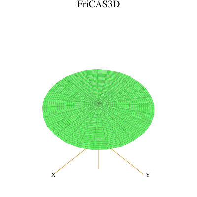
The CoordinateSystems package exports the following operations: bipolar, bipolarCylindrical, cartesian, conical, cylindrical, elliptic, ellipticCylindrical, oblateSpheroidal, parabolic, parabolicCylindrical, paraboloidal, polar, prolateSpheroidal, spherical, and toroidal. Use Browse or the )show system command to get more information.
A three-dimensional graph can be explicitly clipped within the draw command by indicating a minimum and maximum threshold for the given function definition. These thresholds can be defined using the FriCAS min and max functions.
gamma(x,y) == g := Gamma complex(x,y) point [x, y, max( min(real g, 4), -4), argument g]
Here is an example that clips the gamma function in order to eliminate the extreme divergence it creates.
draw(gamma,-%pi..%pi,-%pi..%pi,var1Steps==50,var2Steps==50)
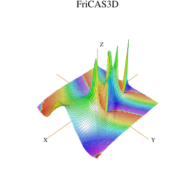
Once you have created a viewport, move your mouse to the viewport and click with your left mouse button. This displays a control-panel on the side of the viewport that is closest to where you clicked.
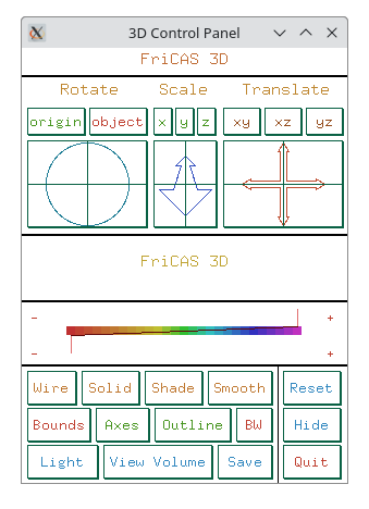
Three-dimensional control-panel.
We recommend you first select the Bounds button while executing transformations since the bounding box displayed indicates the object’s position as it changes.
A rotation transformation occurs by clicking the mouse within the Rotate window in the upper left
corner of the control-panel. The rotation is computed in spherical coordinates, using the horizontal
mouse position to increment or decrement the value of the longitudinal angle  within the
range of 0 to 2
 and the vertical mouse position to increment or decrement the value of
the latitudinal angle

 to
 . The active mode of rotation is
displayed in green on a color monitor or in clear text on a black and white monitor, while
the inactive mode is displayed in red for color display or a mottled pattern for black and
white.
The origin button indicates that the rotation is to occur with respect to the origin of the viewing space, that is indicated by the axes.
The object button indicates that the rotation is to occur with respect to the center of volume of the object, independent of the axes’ origin position.
A scaling transformation occurs by clicking the mouse within the Scale window in the upper center of the control-panel, containing a zoom arrow. The axes along which the scaling is to occur are indicated by selecting the appropriate button above the zoom arrow window. The selected axes are displayed in green on a color monitor or in clear text on a black and white monitor, while the unselected axes are displayed in red for a color display or a mottled pattern for black and white.
Uniform scaling along the x, y and z axes occurs when all the axes buttons are selected.
If any of the axes buttons are not selected, non-uniform scaling occurs, that is, scaling occurs only in the direction of the axes that are selected.
Translation occurs by indicating with the mouse in the Translate window the direction you want the graph to move. This window is located in the upper right corner of the control-panel and contains a potentiometer with crossed arrows pointing up, down, left and right. Along the top of the Translate window are three buttons (XY, XZ, and YZ) indicating the three orthographic projection planes. Each orientates the group as a view into that plane. Any translation of the graph occurs only along this plane.
The window directly below the potentiometer windows for transformations is used to display system messages relating to the viewport, the control-panel and the current graph displaying status.
Directly below the message window is the colormap range indicator window. The FriCAS Colormap shows a sampling of the spectrum from which hues can be drawn to represent the colors of a surface. The Colormap is composed of five shades for each of the hues along this spectrum. By moving the markers above and below the Colormap, the range of hues that are used to color the existing surface are set. The bottom marker shows the hue for the low end of the color range and the top marker shows the hue for the upper end of the range. Setting the bottom and top markers at the same hue results in monochromatic smooth shading of the graph when Smooth mode is selected. At each end of the Colormap are + and - buttons. When clicked on, these increment or decrement the top or bottom marker.
Below the Colormap window and to the left are located various buttons that determine the characteristics of a graph. The buttons along the bottom and right hand side all have special meanings; the remaining buttons in the first row indicate the mode or style used to display the graph. The second row are toggles that turn on or off a property of the graph. On a color monitor, the property is on if green (clear text, on a monochrome monitor) and off if red (mottled pattern, on a monochrome monitor). Here is a list of their functions.
displays surface and tube plots as a wireframe image in a single color (blue) with no hidden surfaces removed, or displays space curve plots in colors based upon their parametric variables. This is the fastest mode for displaying a graph. This is very useful when you want to find a good orientation of your graph.
displays the graph with hidden surfaces removed, drawing each polygon beginning with the furthest from the viewer. The edges of the polygons are displayed in the hues specified by the range in the Colormap window.
displays the graph with hidden surfaces removed and with the polygons shaded, drawing each polygon beginning with the furthest from the viewer. Polygons are shaded in the hues specified by the range in the Colormap window using the Phong illumination model.
displays the graph using a renderer that computes the graph one line at a time. The location and color of the graph at each visible point on the screen are determined and displayed using the Phong illumination model. Smooth shading is done in one of two ways, depending on the range selected in the colormap window and the number of colors available from the hardware and/or window manager. When the top and bottom markers of the colormap range are set to different hues, the graph is rendered by dithering between the transitions in color hue. When the top and bottom markers of the colormap range are set to the same hue, the graph is rendered using the Phong smooth shading model. However, if enough colors cannot be allocated for this purpose, the renderer reverts to the color dithering method until a sufficient color supply is available. For this reason, it may not be possible to render multiple Phong smooth shaded graphs at the same time on some systems.
encloses the entire volume of the viewgraph within a bounding box, or removes the box if previously selected. The region that encloses the entire volume of the viewport graph is displayed.
displays Cartesian coordinate axes of the space, or turns them off if previously selected.
causes quadrilateral polygons forming the graph surface to be outlined in black when the graph is displayed in Shade mode.
converts a color viewport to black and white, or vice-versa. When this button is selected the control-panel and viewport switch to an immutable colormap composed of a range of grey scale patterns or tiles that are used wherever shading is necessary.
takes you to a control-panel described below.
creates a menu of the possible file types that can be written using the control-panel. The Exit button leaves the save menu. The Pixmap button writes an FriCAS pixmap of the current viewport contents. The file is called fricas3D.pixmap and is located in the directory from which FriCAS or viewAlone was started. The PS button writes the current viewport contents to PostScript output rather than to the viewport window. By default the file is called fricas3D.ps; however, if a file name is specified in the user’s .Xdefaults file it is used. The file is placed in the directory from which the FriCAS or viewAlone session was begun. See also the ‘write‘ function.
returns the object transformation characteristics back to their initial states.
causes the control-panel for the corresponding viewport to disappear from the screen.
queries whether the current viewport session should be terminated.
The Light button changes the control-panel into the Lighting Control-Panel. At the top of this panel, the three axes are shown with the same orientation as the object. A light vector from the origin of the axes shows the current position of the light source relative to the object. At the bottom of the panel is an Abort button that cancels any changes to the lighting that were made, and a Return button that carries out the current set of lighting changes on the graph.
The XY lighting axes window is below the Lighting Control-Panel title and to the left. This changes the light vector within the XY view plane.
The Z lighting axis window is below the Lighting Control-Panel title and in the center. This changes the Z location of the light vector.
Below the Lighting Control-Panel title and to the right is the light intensity meter. Moving the intensity indicator down decreases the amount of light emitted from the light source. When the indicator is at the top of the meter the light source is emitting at 100% intensity. At the bottom of the meter the light source is emitting at a level slightly above ambient lighting.
The View Volume button changes the control-panel into the Viewing Volume Panel. At the bottom of the viewing panel is an Abort button that cancels any changes to the viewing volume that were made and a Return button that carries out the current set of viewing changes to the graph.
At the top of this panel is the Eye Reference window. It shows a planar projection of the viewing pyramid from the eye of the viewer relative to the location of the object. This has a bounding region represented by the rectangle on the left. Below the object rectangle is the Hither window. By moving the slider in this window the hither clipping plane sets the front of the view volume. As a result of this depth clipping all points of the object closer to the eye than this hither plane are not shown. The Eye Distance slider to the right of the Hither slider is used to change the degree of perspective in the image.
The Clip Volume window is at the bottom of the Viewing Volume Panel. On the right is a Settings menu. In this menu are buttons to select viewing attributes. Selecting the Perspective button computes the image using perspective projection. The Show Region button indicates whether the clipping region of the volume is to be drawn in the viewport and the Clipping On button shows whether the view volume clipping is to be in effect when the image is drawn. The left side of the Clip Volume window shows the clipping boundary of the graph. Moving the knobs along the X, Y, and Z sliders adjusts the volume of the clipping region accordingly.
Here is a summary of useful FriCAS operations for three-dimensional graphics. Each operation name is followed by a list of arguments. Each argument is written as a variable informally named according to the type of the argument (for example, integer). If appropriate, a default value for an argument is given in parentheses immediately following the name.
()
tests whether space curves are to be plotted according to the adaptive refinement algorithm.
(viewport,  (1),
 (27))
sets the colormap range to be from  to
 .
(viewport, string("off"))
declares whether the control-panel for the viewport is to be displayed or not.
(viewport, string("off"))
declares whether the polygon outline includes the diagonals or not.
(viewport, style)
selects which of four drawing styles are used: "wireMesh", "solid", "shade", or "smooth".
(viewport,float(500))
sets the distance of the eye from the origin of the object for use in the ‘perspective‘.
(viewport)
returns the operating system process ID number for the viewport.
(viewport,  (-0.5),
 (0.5),
 (0.5))
sets the Cartesian coordinates of the light source.
(viewport,integer,point)
replaces the coordinates of the point with the index integer with point.
(viewport,  (viewPosDefault),
 (viewPosDefault))
moves the upper left-hand corner of the viewport to screen position ( ,
 ).
(viewport)
returns a list of all current draw options.
(viewport, string("off"))
turns polygon outlining off or on when drawing in "shade" mode.
(viewport, string("on"))
turns perspective viewing on and off.
(viewport)
resets the attributes of a viewport to their initial settings.
(viewport,  (viewSizeDefault),
 (viewSizeDefault))
resets the width and height values for a viewport.
(viewport,  (viewThetaDefault),
 (viewPhiDefault))
rotates the viewport by rotation angles for longitude ( ) and latitude (
 ). Angles designate
radians if given as floats, or degrees if given as integers.
(boolean(true))
sets whether space curves are to be plotted according to the adaptive refinement algorithm.
(integer(1000))
sets the default maximum number of possible points to be used when constructing a
three-dimensional space curve.
(integer(49))
sets the default minimum number of possible points to be used when constructing a
three-dimensional space curve.
(integer(500))
sets the default screen resolution constant used in setting the computation limit of adaptively
generated three-dimensional space curve plots.
(viewport, string("off"))
declares whether the bounding box of a graph is shown or not.
(viewport)
returns the space component.
(viewport, subspace)
resets the space component to subspace.
(viewport,  (viewDeltaXDefault),
 (viewDeltaYDefault))
translates the object horizontally and vertically relative to the center of the viewport.
(viewport,float(1.0))
resets the intensity I of the light source, 
([integer(6)])
sets or indicates the default number of vertices defining the polygon that is used to create a tube
around a space curve.
([float(0.5)])
sets or indicates the default radius of the tube that encircles a space curve.
([integer(27)])
sets or indicates the default number of increments into which the grid defining a surface plot is
subdivided with respect to the first parameter declared in the surface function.
([integer(27)])
sets or indicates the default number of increments into which the grid defining a surface plot is
subdivided with respect to the second parameter declared in the surface function.
([ ,
 ,
 ,
 ,
 ,
 ,
 ])
resets the default settings for the point color, line color, axes color, units color, point size,
viewport upper left-hand corner position, and the viewport size.
([float(0)])
resets the default horizontal offset from the center of the viewport, or returns the current default
offset if no argument is given.
([float(0)])
resets the default vertical offset from the center of the viewport, or returns the current default
offset if no argument is given.
([float(- /4)])
resets the default latitudinal view angle, or returns the current default angle if no argument is
given.  is set to this value.
(viewport,  ,
 ,
 )
sets the viewing position in Cartesian coordinates.
(viewport,  ,
 )
sets the viewing position in spherical coordinates.
(viewport,  ,
 ,
 ,
 ,
 )
sets the viewing position in spherical coordinates, the scale factor, and offsets.  (longitude)
and
 (latitude) are in radians.
([list([0,0])])
sets or indicates the position of the upper left-hand corner of a two-dimensional viewport, relative
to the display root window (the upper left-hand corner of the display is [0, 0]).
([list([400,400])])
sets or indicates the width and height dimensions of a viewport.
([float( /4)])
resets the default longitudinal view angle, or returns the current default angle if no argument is
given. When a parameter is specified, the default longitudinal view angle  is set to this value.
([list(["pixmap", "bitmap", "postscript", "image")])
indicates the possible file types that can be created with the ‘write‘ function.
([list([])])
sets or indicates the default types of files that are created in addition to the data file when a
‘write‘ command is executed on a viewport.
(viewport, directory, [option])
writes the file data for viewport in the directory directory. An optional third argument specifies
a file type (one of pixmap, bitmap, postscript, or image), or a list of file types. An additional
file is written for each file type listed.
Both the two-dimensional and three-dimensional drawing facilities consult the .Xdefaults file for various defaults. The list of defaults that are recognized by the graphing routines is discussed in this section. These defaults are preceded by FriCAS.3D. for three-dimensional viewport defaults, FriCAS.2D. for two-dimensional viewport defaults, or FriCAS* (no dot) for those defaults that are acceptable to either viewport type.
This indicates which font type is used for the button text on the control-panel. The default value
is "Rom11".
(2D only)
This indicates which font type is used for displaying the graph numbers and slots in the Graphs
section of the two-dimensional control-panel. The default value is "Rom22".
This indicates which font type is used for the axes labels and potentiometer header names on
three-dimensional viewport windows. This is also used for two-dimensional control-panels for
indicating which font type is used for potentiometer header names and multiple graph title
headers. The default value is "Itl14".
This indicates whether the background color is to be inverted from white to black. If on, the
graph viewports use black as the background color. If off or no declaration is made, the graph
viewports use a white background. The default value is "off".
(3D only)
This indicates which font type is used for the x, y, and z labels of the two lighting axes
potentiometers, and for the Intensity title on the lighting control-panel. The default value is
"Rom10".
These indicate the font type to be used for the text in the control-panel message window. The
default value is "Rom14".
This indicates whether the graph viewports are to be displayed as if the monitor is black and
white, that is, a 1 bit plane. If on is specified, the viewport display is black and white. If off is
specified, or no declaration for this default is given, the viewports are displayed in the normal
fashion for the monitor in use. The default value is "off".
This indicates which font type is used for the title text and, for three-dimensional graphs, in the
lighting and viewing-volume control-panel windows. The default value is "Rom14".
(2D only)
This indicates which font type is used for displaying the unit labels on two-dimensional viewport
graphs. The default value is "6x10".
(3D only)
This indicates which font type is used for the x, y, and z labels of the clipping region sliders;
for the Perspective, Show Region, and Clipping On buttons under Settings, and above
the windows for the Hither and Eye Distance sliders in the Viewing Volume Panel of the
three-dimensional control-panel. The default value is "Rom8".
In this chapter we describe techniques useful in solving advanced problems with FriCAS.
FriCAS provides two basic floating-point types: Float and DoubleFloat. This section describes how to use numerical operations defined on these types and the related complex types. As we mentioned in Chapter 1, the Float type is a software implementation of floating-point numbers in which the exponent and the significand may have any number of digits. See ‘Float’ on page 895 for detailed information about this domain. The DoubleFloat (see ‘DoubleFloat’ on page 833) is usually a hardware implementation of floating point numbers, corresponding to machine double precision. The types Complex Float and Complex DoubleFloat are the corresponding software implementations of complex floating-point numbers. In this section the term floating-point type means any of these four types. The floating-point types implement the basic elementary functions. These include (where “%” means DoubleFloat, Float, Complex DoubleFloat, or Complex Float):
exp, log: %  %
sin, cos, tan, cot, sec, csc: %  %
asin, acos, atan, acot, asec, acsc: %  %
sinh, cosh, tanh, coth, sech, csch: %  %
asinh, acosh, atanh, acoth, asech, acsch: %  %
pi: ()  %
sqrt: %  %
nthRoot: (%, Integer)  %
^: (%, Fraction Integer)  %
^: (%, %)  %
The handling of roots depends on whether the floating-point type is real or complex: for the real
floating-point types, DoubleFloat and Float, if a real root exists the one with the same sign as
the radicand is returned; for the complex floating-point types, the principal value is returned.
Also, for real floating-point types the inverse functions produce errors if the results are not real.
This includes cases such as asin(1.2), log(-3.2), sqrt(-1.1). The default floating-point
type is Float so to evaluate functions using Float or Complex Float, just use normal decimal
notation.
exp(3.1)
exp(3.1 + 4.5 * %i)
Complex(Float) To evaluate functions using DoubleFloat or Complex DoubleFloat, a declaration or conversion is required.
r: DFLOAT := 3.1; t: DFLOAT := 4.5; exp(r + t*%i)
exp(3.1::DFLOAT + 4.5::DFLOAT * %i)
Complex(DoubleFloat) A number of special functions are provided by the package DoubleFloatSpecialFunctions
for the machine-precision floating-point types. The special functions provided are listed below, where F stands
for the types DoubleFloat and Complex DoubleFloat. The real versions of the functions yield an error if
the result is not real.
Gamma: F  F
Gamma(z) is the Euler gamma function,  , defined by
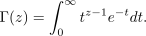
Beta: F  F
Beta(u, v) is the Euler Beta function,  , defined by

This is related to  by
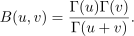
logGamma: F  F
logGamma(z) is the natural logarithm of  . This can often be computed even if
 cannot.
digamma: F  F
digamma(z), also called psi(z), is the function  , defined by

polygamma: (NonNegativeInteger, F)  F
polygamma(n, z) is the  derivative of
 , written
 .
besselJ: (F,F)  F
besselJ(v,z) is the Bessel function of the first kind,  . This function satisfies the differential
equation

besselY: (F,F)  F
besselY(v,z) is the Bessel function of the second kind,  . This function satisfies the same differential
equation as besselJ. The implementation simply uses the relation

besselI: (F,F)  F
besselI(v,z) is the modified Bessel function of the first kind,  . This function satisfies the differential
equation

besselK: (F,F)  F
besselK(v,z) is the modified Bessel function of the second kind,  . This function satisfies the same
differential equation as besselI. The implementation simply uses the relation
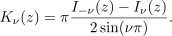
airyAi: F  F
airyAi(z) is the Airy function  . This function satisfies the differential equation
 The implementation simply uses the relation

airyBi: F  F
airyBi(z) is the Airy function  . This function satisfies the same differential equation as airyAi. The
implementation simply uses the relation

hypergeometric0F1: (F,F)  F
hypergeometric0F1(c,z) is the hypergeometric function  .
The package FloatSpecialFunctions provides the implementation of some special functions for Float or Complex Float arguments, including Gamma, Beta, logGamma, digamma. If you give Float or Complex Float arguments to a special function that has not yet been defined to accept Float arguments, these are respectively converted to DoubleFloat or Complex DoubleFloat arguments.
Gamma(0.5)^2
a := 2.1; b := 1.1; besselI(a + %i*b, b*a + 1)
Complex(DoubleFloat) A number of additional operations may be used to compute numerical values. These are
special polynomial functions that can be evaluated for values in any commutative ring R, and in
particular for values in any floating-point type. The following operations are provided by the package
OrthogonalPolynomialFunctions:
chebyshevT: (NonNegativeInteger, R)  R
chebyshevT(n,z) is the  Chebyshev polynomial of the first kind,
 . These are defined
by
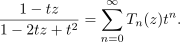
chebyshevU: (NonNegativeInteger, R)  R
chebyshevU(n,z) is the  Chebyshev polynomial of the second kind,
 . These are defined
by
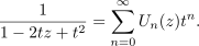
hermiteH: (NonNegativeInteger, R)  R
hermiteH(n,z) is the  Hermite polynomial,
 . These are defined by
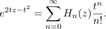
laguerreL: (NonNegativeInteger, R)  R
laguerreL(n,z) is the  Laguerre polynomial,
 . These are defined by
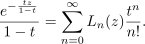
laguerreL: (NonNegativeInteger, NonNegativeInteger, R)  R
laguerreL(m,n,z) is the associated Laguerre polynomial,  . This is the
 derivative of
 .
legendreP: (NonNegativeInteger, R)  R
legendreP(n,z) is the  Legendre polynomial,
 . These are defined by
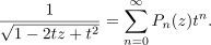
These operations require non-negative integers for the indices, but otherwise the argument can be given as desired.
[chebyshevT(i, z) for i in 0..5]
List(Polynomial(Integer)) The expression chebyshevT(n,z) evaluates to the  Chebyshev polynomial of the first
kind.
chebyshevT(3, 5.0 + 6.0*%i)
chebyshevT(3, 5.0::DoubleFloat)
DoubleFloat The expression chebyshevU(n,z) evaluates to the  Chebyshev polynomial of the second
kind.
[chebyshevU(i, z) for i in 0..5]
chebyshevU(3, 0.2)
Float The expression hermiteH(n,z) evaluates to the  Hermite polynomial.
[hermiteH(i, z) for i in 0..5]
hermiteH(100, 1.0)
Float The expression laguerreL(n,z) evaluates to the  Laguerre polynomial.
[laguerreL(i, z) for i in 0..4]
laguerreL(4, 1.2)
[laguerreL(j, 3, z) for j in 0..4]
laguerreL(1, 3, 2.1)
Float The expression legendreP(n,z) evaluates to the  Legendre polynomial,
[legendreP(i,z) for i in 0..5]
List(Polynomial(Fraction(Integer)))
legendreP(3, 3.0*%i)
Finally, three number-theoretic polynomial operations may be evaluated. The following operations are provided by the package NumberTheoreticPolynomialFunctions. .
bernoulliB: (NonNegativeInteger, R)  R
bernoulliB(n,z) is the  Bernoulli polynomial,
 . These are defined by
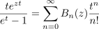
eulerE: (NonNegativeInteger, R)  R
eulerE(n,z) is the  Euler polynomial,
 . These are defined by
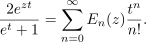
cyclotomic: (NonNegativeInteger, R)  R
cyclotomic(n,z) is the  cyclotomic polynomial
 . This is the polynomial whose roots are precisely
the primitive
 roots of unity. This polynomial has degree given by the Euler totient function
 .
The expression bernoulliB(n,z) evaluates to the  Bernoulli polynomial.
bernoulliB(3, z)
bernoulliB(3, 0.7 + 0.4 * %i)
Complex(Float) The expression eulerE(n,z) evaluates to the  Euler polynomial.
eulerE(3, z)
eulerE(3, 0.7 + 0.4 * %i)
Complex(Float) The expression cyclotomic(n,z) evaluates to the  cyclotomic polynomial.
cyclotomic(3, z)
cyclotomic(3, (-1.0 + 0.0 * %i)^(2/3))
Drawing complex functions in FriCAS is presently somewhat awkward compared to drawing real functions. It is necessary to use the draw operations that operate on functions rather than expressions.
This is the complex exponential function (rotated interactively). When this is displayed in color, the height is the value of the real part of the function and the color is the imaginary part. Red indicates large negative imaginary values, green indicates imaginary values near zero and blue/violet indicates large positive imaginary values.
draw((x,y)+-> real exp complex(x,y), -2..2, -2*%pi..2*%pi, colorFunction == (x, y) +-> imag exp complex(x,y), title=="exp(x+%i*y)", style=="smooth")
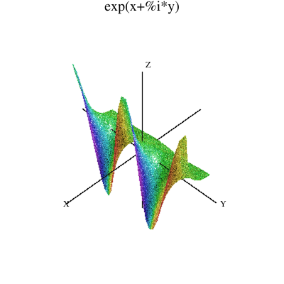
This is the complex arctangent function. Again, the height is the real part of the function value but here the color indicates the function value’s phase. The position of the branch cuts are clearly visible and one can see that the function is real only for a real argument.
vp := draw((x,y) +-> real atan complex(x,y), -%pi..%pi, -%pi..%pi, colorFunction==(x,y) +->argument atan complex(x,y), title=="atan(x+%i*y)", style=="shade"); rotate(vp,-160,-45); vp
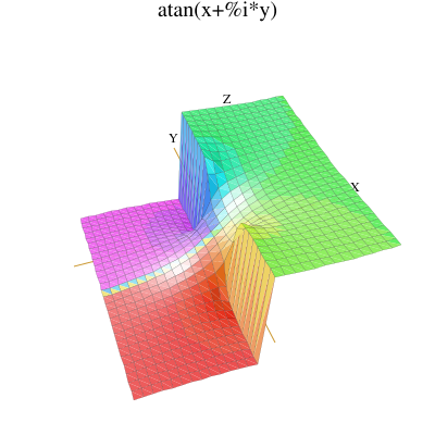
This is the complex Gamma function.
draw((x,y) +-> max(min(real Gamma complex(x,y),4),-4), -%pi..%pi, -%pi..%pi, style=="shade", colorFunction == (x,y) +-> argument Gamma complex(x,y), title == "Gamma(x+%i*y)", var1Steps == 50, var2Steps== 50)
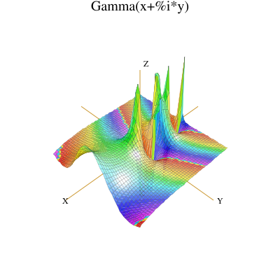
This shows the real Beta function near the origin.
draw(Beta(x,y)/100, x=-1.6..1.7, y = -1.6..1.7, style=="shade", title=="Beta(x,y)", var1Steps==40, var2Steps==40)
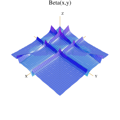
This is the Bessel function  for index
 in the range
-6..4 and argument  in the range
2..14.
draw((alpha,x) +-> min(max(besselJ(alpha, x+8), -6), 6), -6..4, -6..6, title=="besselJ(alpha,x)", style=="shade", var1Steps==40, var2Steps==40)
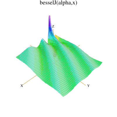
This is the modified Bessel function  evaluated for various real values of the index
 and fixed
argument
 .
draw(besselI(alpha, 5), alpha = -12..12, unit==[5,20])
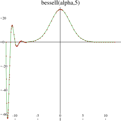
This is similar to the last example except the index  takes on complex values in a
6 x 6 rectangle centered on
the origin.
draw((x,y) +-> real besselI(complex(x/20, y/20),5), -60..60, -60..60, colorFunction == (x,y)+-> argument besselI(complex(x/20,y/20),5), title=="besselI(x+i*y,5)", style=="shade")
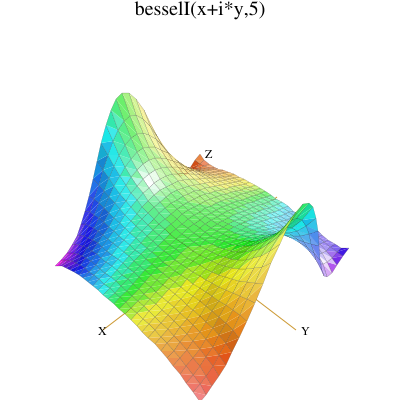
The FriCAS polynomial factorization facilities are available for all polynomial types and a wide variety of coefficient domains. Here are some examples.
Polynomials with integer coefficients can be factored.
v := (4*x^3+2*y^2+1)*(12*x^5-x^3*y+12)
factor v
Factored(Polynomial(Integer)) Also, FriCAS can factor polynomials with rational number coefficients.
w := (4*x^3+(2/3)*x^2+1)*(12*x^5-(1/2)*x^3+12)
factor w
Factored(Polynomial(Fraction(Integer)))
Polynomials with coefficients in a finite field can be also be factored.
u : POLY(PF(19)) :=3*x^4+2*x^2+15*x+18
Polynomial(PrimeField(19)) These include the integers mod p, where p is prime, and extensions of these
fields.
factor u
Factored(Polynomial(PrimeField(19))) Convert this to have coefficients in the finite field with  elements. See Section 8.11 on
page 599 for more information about finite fields.
factor(u :: POLY FFX(PF 19,3))
Factored(Polynomial(FiniteFieldExtension(PrimeField(19), 3)))
Polynomials with coefficients in simple algebraic extensions of the rational numbers can be factored.
Here, aa and bb are symbolic roots of polynomials.
aa := rootOf(aa^2+aa+1)
p:=(x^3+aa^2*x+y)*(aa*x^2+aa*x+aa*y^2)^2
Polynomial(AlgebraicNumber) Note that the second argument to factor can be a list of algebraic extensions to factor over.
factor(p,[aa])
Factored(Polynomial(AlgebraicNumber)) This factors x^2+3 over the integers.
factor(x^2+3)
Factored(Polynomial(Integer)) Factor the same polynomial over the field obtained by adjoining aa to the rational
numbers.
factor(x^2+3,[aa])
Factored(Polynomial(AlgebraicNumber)) Factor x^6+108 over the same field.
factor(x^6+108,[aa])
Factored(Polynomial(AlgebraicNumber))
bb:=rootOf(bb^3-2)
factor(x^6+108,[bb])
Factored(Polynomial(AlgebraicNumber)) Factor again over the field obtained by adjoining both aa and bb to the rational
numbers.
factor(x^6+108,[aa,bb])
Factored(Polynomial(AlgebraicNumber))
Since fractions of polynomials form a field, every element (other than zero) divides any other, so there is no useful notion of irreducible factors. Thus the factor operation is not very useful for fractions of polynomials.
There is, instead, a specific operation factorFraction that separately factors the numerator and denominator and returns a fraction of the factored results.
factorFraction((x^2-4)/(y^2-4))
Fraction(Factored(Polynomial(Integer))) You can also use map. This expression applies the factor operation to the numerator and denominator.
map(factor,(x^2-4)/(y^2-4))
Fraction(Factored(Polynomial(Integer)))
In this section we show you how to work with one root or all roots of a polynomial. These roots are represented symbolically (as opposed to being numeric approximations). See Section 8.5.2 on page 526 and Section 8.5.3 on page 529 for information about solving for the roots of one or more polynomials.
Use rootOf to get a symbolic root of a polynomial: rootOf(p, x) returns a root of p(x).
This creates an algebraic number a.
a := rootOf(a^4+1,a)
Expression(Integer) To find the algebraic relation that defines a, use definingPolynomial.
definingPolynomial a
Expression(Integer) You can use a in any further expression, including a nested rootOf.
b := rootOf(b^2-a-1,b)
Expression(Integer) Higher powers of the roots are automatically reduced during calculations.
a + b
% ^ 5
Expression(Integer) The operation zeroOf is similar to rootOf, except that it may express the root using radicals in some cases.
rootOf(c^2+c+1,c)
zeroOf(d^2+d+1,d)
rootOf(e^5-2,e)
zeroOf(f^5-2,f)
Use rootsOf to get all symbolic roots of a polynomial: rootsOf(p, x) returns a list of all the roots of p(x). If
p(x) has a multiple root of order n, then that root appears n times in the list.
Compute all the roots of x^4 + x + 1.
l := rootsOf(x^4 + x + 1,x)
List(Expression(Integer)) As a side effect, the variables %x0, %x1 and %x2 are bound to the first three roots of
x^4 + x + 1.
%x0^5
Expression(Integer) Although they all satisfy x^4 + x + 1 = 0, %x0, %x1, and %x2 are different algebraic numbers.
To find the algebraic relation that defines each of them, use definingPolynomial.
definingPolynomial %x0
definingPolynomial %x1
definingPolynomial %x2
Expression(Integer) We can check that the sum and product of the roots of x^4 + x + 1 are its trace and
norm.
x3 := last l
%x0 + %x1 + %x2 + x3
%x0 * %x1 * %x2 * x3
Expression(Integer) Note, that in general roots are expressions in new symbols. For example for x^4 + 1 the
second root is a product.
rootsOf(x^4 + 1, x)
List(Expression(Integer)) Corresponding to the pair of operations rootOf/zeroOf in Section 8.5.2 on page 526, there is an operation zerosOf that, like rootsOf, computes all the roots of a given polynomial, but which expresses some of them in terms of radicals.
zerosOf(y^4 + y + 1, y)
List(Expression(Integer)) As you see, only two implicit algebraic numbers were created (%y0,%y1), and its defining
equations are below. The other two roots are expressed in radicals.
definingPolynomial %y0
definingPolynomial %y1
Expression(Integer) For x^4 + 1 all roots can be expressed in radicals.
zerosOf(x^4 + 1)
In this section we show you some of FriCAS’s facilities for computing and manipulating eigenvalues and eigenvectors, also called characteristic values and characteristic vectors, respectively.
Let’s first create a matrix with integer entries.
m1 := matrix [[1,2,1],[2,1,-2],[1,-2,4]]
Matrix(Integer) To get a list of the rational eigenvalues, use the operation eigenvalues.
leig := eigenvalues(m1)
List(Union(Fraction(Polynomial(Integer)), SuchThat(Symbol, Polynomial(Integer)))) Given an explicit eigenvalue, eigenvector computes the eigenvectors corresponding to it.
eigenvector(first(leig),m1)
List(Matrix(Fraction(Polynomial(Fraction(Integer)))))
The operation eigenvectors returns a list of pairs of values and vectors. When an eigenvalue is rational, FriCAS gives you the value explicitly; otherwise, its minimal polynomial is given, (the polynomial of lowest degree with the eigenvalues as roots), together with a parametric representation of the eigenvector using the eigenvalue. This means that if you ask FriCAS to solve the minimal polynomial, then you can substitute these roots into the parametric form of the corresponding eigenvectors.
You must be aware that unless an exact eigenvalue has been computed, the eigenvector may be badly in error.
eigenvectors(m1)
List(Record(eigval: Union(Fraction(Polynomial(Integer)), SuchThat(Symbol, Polynomial(Integer))), eigmult: NonNegativeInteger, eigvec: List(Matrix(Fraction(Polynomial(Integer)))))) Another possibility is to use the operation radicalEigenvectors, which tries to compute explicitly the eigenvectors in terms of radicals.
radicalEigenvectors(m1)
Alternatively, FriCAS can compute real or complex approximations to the eigenvectors and eigenvalues using
the operations realEigenvectors or complexEigenvectors. They each take an additional argument  to specify
the “precision” required. In the real case, this means that each approximation will be within
 of the
actual result. In the complex case, this means that each approximation will be within
 of the actual
result in each of the real and imaginary parts.
The precision can be specified as a Float if the results are desired in floating-point notation, or as Fraction Integer if the results are to be expressed using rational (or complex rational) numbers.
realEigenvectors(m1,1/1000)
List(Record(outval: Fraction(Integer), outmult: Integer, outvect: List(Matrix(Fraction(Integer))))) If an n by n matrix has n distinct eigenvalues (and therefore n eigenvectors) the operation
eigenMatrix gives you a matrix of the eigenvectors.
eigenMatrix(m1)
Union(Matrix(Expression(Integer)), ...)
m2 := matrix [[-5,-2],[18,7]]
eigenMatrix(m2)
Union("failed", ...) If a symmetric matrix has a basis of orthonormal eigenvectors, then orthonormalBasis computes a list of these vectors.
m3 := matrix [[1,2],[2,1]]
orthonormalBasis(m3)
List(Matrix(Expression(Integer)))
In this section we discuss the FriCAS facilities for solving systems of linear equations, finding the roots of polynomials and solving systems of polynomial equations. For a discussion of the solution of differential equations, see Section 8.10 on page 581.
You can use the operation solve to solve systems of linear equations.
The operation solve takes two arguments, the list of equations and the list of the unknowns to be solved for. A system of linear equations need not have a unique solution.
To solve the linear system:
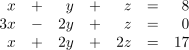
evaluate this expression.
solve([x+y+z=8,3*x-2*y+z=0,x+2*y+2*z=17],[x,y,z])
List(List(Equation(Fraction(Polynomial(Integer)))))
Parameters are given as new variables starting with a percent sign and “%” and the variables are expressed in terms of the parameters. If the system has no solutions then the empty list is returned.
When you solve the linear system
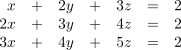
with this expression you get a solution involving a parameter.
solve([x+2*y+3*z=2,2*x+3*y+4*z=2,3*x+4*y+5*z=2],[x,y,z])
List(List(Equation(Fraction(Polynomial(Integer)))))
The system can also be presented as a matrix and a vector. The matrix contains the coefficients of the linear equations and the vector contains the numbers appearing on the right-hand sides of the equations. You may input the matrix as a list of rows and the vector as a list of its elements.
To solve the system:
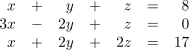
in matrix form you would evaluate this expression.
solve([[1,1,1],[3,-2,1],[1,2,2]],[8,0,17])
The solutions are presented as a Record with two components: the component particular contains a particular solution of the given system or the item "failed" if there are no solutions, the component basis contains a list of vectors that are a basis for the space of solutions of the corresponding homogeneous system. If the system of linear equations does not have a unique solution, then the basis component contains non-trivial vectors.
This happens when you solve the linear system
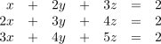
with this command.
solve([[1,2,3],[2,3,4],[3,4,5]],[2,2,2])
All solutions of this system are obtained by adding the particular solution with a linear combination of the basis vectors.
When no solution exists then "failed" is returned as the particular component.
For example:
solve([[1,2,3],[2,3,4],[3,4,5]],[2,3,2])
When you want to solve a system of homogeneous equations (that is, a system where the numbers on the right-hand sides of the equations are all zero) in the matrix form you can omit the second argument and use the nullSpace operation.
This computes the solutions of the following system of equations:
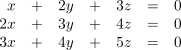
The result is given as a list of vectors and these vectors form a basis for the solution space.
nullSpace([[1,2,3],[2,3,4],[3,4,5]])
FriCAS can solve polynomial equations producing either approximate or exact solutions. Exact solutions are either members of the ground field or can be presented symbolically as roots of irreducible polynomials.
This returns the one rational root along with an irreducible polynomial describing the other solutions.
solve(x^3 = 8,x)
List(Equation(Fraction(Polynomial(Integer)))) If you want solutions expressed in terms of radicals you would use this instead.
radicalSolve(x^3 = 8,x)
List(Equation(Expression(Integer)))
The solve command always returns a value but radicalSolve returns only the solutions that it is able to express in terms of radicals.
If the polynomial equation has rational coefficients you can ask for approximations to its real roots by calling
solve with a second argument that specifies the “precision”  . This means that each approximation will be
within
 of the actual result.
Notice that the type of second argument controls the type of the result.
solve(x^4 - 10*x^3 + 35*x^2 - 50*x + 25,.0001)
List(Equation(Polynomial(Float))) If you give a floating-point precision you get a floating-point result; if you give the precision as a rational number you get a rational result.
solve(x^3-2,1/1000)
List(Equation(Polynomial(Fraction(Integer)))) If you want approximate complex results you should use the command complexSolve that takes
the same precision argument  .
complexSolve(x^3-2,.0001)
List(Equation(Polynomial(Complex(Float)))) Each approximation will be within  of the actual result in each of the real and imaginary
parts.
complexSolve(x^2-2*%i+1,1/100)
List(Equation(Polynomial(Complex(Fraction(Integer)))))
Note that if you omit the = from the first argument FriCAS generates an equation by equating the first argument to zero. Also, when only one variable is present in the equation, you do not need to specify the variable to be solved for, that is, you can omit the second argument.
FriCAS can also solve equations involving rational functions. Solutions where the denominator vanishes are discarded.
radicalSolve(1/x^3 + 1/x^2 + 1/x = 0,x)
List(Equation(Expression(Integer)))
Given a system of equations of rational functions with exact coefficients:

FriCAS can find numeric or symbolic solutions. The system is first split into irreducible components, then for each component, a triangular system of equations is found that reduces the problem to sequential solution of univariate polynomials resulting from substitution of partial solutions from the previous stage.

Symbolic solutions can be presented using “implicit” algebraic numbers defined as roots of irreducible polynomials or in terms of radicals. FriCAS can also find approximations to the real or complex roots of a system of polynomial equations to any user-specified accuracy.
The operation solve for systems is used in a way similar to solve for single equations. Instead of a polynomial equation, one has to give a list of equations and instead of a single variable to solve for, a list of variables. For solutions of single equations see Section 8.5.2 on page 526.
Use the operation solve if you want implicitly presented solutions.
solve([3*x^3 + y + 1,y^2 -4],[x,y])
List(List(Equation(Fraction(Polynomial(Integer)))))
solve([x = y^2-19,y = z^2+x+3,z = 3*x],[x,y,z])
List(List(Equation(Fraction(Polynomial(Integer))))) Use radicalSolve if you want your solutions expressed in terms of radicals.
radicalSolve([3*x^3 + y + 1,y^2 -4],[x,y])
List(List(Equation(Expression(Integer))))
To get numeric solutions you only need to give the list of equations and the precision desired. The list of variables would be redundant information since there can be no parameters for the numerical solver.
If the precision is expressed as a floating-point number you get results expressed as floats.
solve([x^2*y - 1,x*y^2 - 2],.01)
List(List(Equation(Polynomial(Float)))) To get complex numeric solutions, use the operation complexSolve, which takes the same arguments as in the real case.
complexSolve([x^2*y - 1,x*y^2 - 2],1/1000)
List(List(Equation(Polynomial(Complex(Fraction(Integer)))))) It is also possible to solve systems of equations in rational functions over the rational
numbers. Note that [x = 0.0, a = 0.0] is not returned as a solution since the denominator vanishes
there.
solve([x^2/a = a,a = a*x],.001)
List(List(Equation(Polynomial(Float)))) When solving equations with denominators, all solutions where the denominator vanishes are discarded.
radicalSolve([x^2/a + a + y^3 - 1,a*y + a + 1],[x,y])
List(List(Equation(Expression(Integer))))
To compute a limit, you must specify a functional expression, a variable, and a limiting value for that variable. If you do not specify a direction, FriCAS attempts to compute a two-sided limit.
Issue this to compute the limit
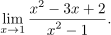
limit((x^2 - 3*x + 2)/(x^2 - 1),x = 1)
Union(OrderedCompletion(Fraction(Polynomial(Integer))), ...)
Sometimes the limit when approached from the left is different from the limit from the right and, in this case, you may wish to ask for a one-sided limit. Also, if you have a function that is only defined on one side of a particular value, you can compute a one-sided limit.
The function log(x) is real only to the right of zero, that is, for x > 0. Thus, when computing limits of
functions involving log(x), you probably want a “right-hand” limit.
limit(x * log(x),x = 0,"right")
Union(OrderedCompletion(Expression(Integer)), ...) When you do not specify "right" or "left" as the optional fourth argument, limit tries to
compute a two-sided limit. Here the limit from the left does not exist, as FriCAS indicates when you try to
take a two-sided limit.
limit(sin(1/x)*exp(1/x), x=0)
A function can be defined on both sides of a particular value, but tend to different limits as its variable
approaches that value from the left and from the right. We can construct an example of this as follows: Since
 is simply the absolute value of
y, the function  is simply the sign (
+1 or -1) of the nonzero real
number y. Therefore,  for
y < 0 and  for
y > 0. This is what happens when we take
the limit at y = 0. The answer returned by FriCAS gives both a “left-hand” and a “right-hand”
limit.
limit(sqrt(y^2)/y,y = 0)
Union(Record(leftHandLimit: Union(OrderedCompletion(Expression(Integer)), "failed"), rightHandLimit: Union(OrderedCompletion(Expression(Integer)), "failed")), ...) Here is another example, this time using a more complicated function.
limit(sqrt(1 - cos(t))/t,t = 0)
You can compute limits at infinity by passing either  or
 as the third argument of limit. To do
this, use the constants
%plusInfinity and %minusInfinity.
limit(sqrt(3*x^2 + 1)/(5*x),x = %plusInfinity)
Union(OrderedCompletion(Expression(Integer)), ...)
limit(sqrt(3*x^2 + 1)/(5*x),x = %minusInfinity)
Union(OrderedCompletion(Expression(Integer)), ...)
You can take limits of functions with parameters. As you can see, the limit is expressed in terms of the parameters.
limit(sinh(a*x)/tan(b*x),x = 0)
Union(OrderedCompletion(Expression(Integer)), ...)
When you use limit, you are taking the limit of a real function of a real variable. When you compute this,
FriCAS returns 0 because, as a function of a real variable, sin(1/z) is always between -1 and 1, so
z * sin(1/z) tends to 0 as z tends to 0.
limit(z * sin(1/z),z = 0)
Union(OrderedCompletion(Expression(Integer)), ...) However, as a function of a complex variable, sin(1/z) is badly behaved near 0 (one says
that sin(1/z) has an essential singularity at z = 0). When viewed as a function of a complex variable,
z * sin(1/z) does not approach any limit as z tends to 0 in the complex plane. FriCAS indicates this when we
call complexLimit.
complexLimit(z * sin(1/z),z = 0)
You can also take complex limits at infinity, that is, limits of a function of z as z approaches infinity on the
Riemann sphere. Use the symbol %infinity to denote “complex infinity.” As above, to compute complex
limits rather than real limits, use complexLimit.
complexLimit((2 + z)/(1 - z),z = %infinity)
OnePointCompletion(Fraction(Polynomial(Integer))) In many cases, a limit of a real function of a real variable exists when the corresponding complex limit does not. This limit exists.
limit(sin(x)/x,x = %plusInfinity)
Union(OrderedCompletion(Expression(Integer)), ...) But this limit does not.
complexLimit(sin(x)/x,x = %infinity)
FriCAS can compute some forward Laplace transforms, mostly of elementary functions not involving
logarithms, although some cases of special functions are handled. To compute the forward Laplace transform
of F(t) with respect to t and express the result as f(s), issue the command laplace(F(t), t, s).
laplace(sin(a*t)*cosh(a*t)-cos(a*t)*sinh(a*t), t, s)
Expression(Integer) Here are some other non-trivial examples.
laplace((exp(a*t) - exp(b*t))/t, t, s)
laplace(2/t * (1 - cos(a*t)), t, s)
laplace(exp(-a*t) * sin(b*t) / b^2, t, s)
laplace((cos(a*t) - cos(b*t))/t, t, s)
Expression(Integer) FriCAS also knows about a few special functions.
laplace(exp(a*t+b)*Ei(c*t), t, s)
laplace(a*Ci(b*t) + c*Si(d*t), t, s)
Expression(Integer) When FriCAS does not know about a particular transform, it keeps it as a formal transform in the answer.
laplace(sin(a*t) - a*t*cos(a*t) + exp(t^2), t, s)
Integration is the reverse process of differentiation, that is, an integral of a function f with respect to a
variable x is any function g such that D(g,x) is equal to f. The package FunctionSpaceIntegration
provides the top-level integration operation, integrate, for integrating real-valued elementary functions.
integrate(cosh(a*x)*sinh(a*x), x)
Union(Expression(Integer), ...) Unfortunately, antiderivatives of most functions cannot be expressed in terms of elementary functions.
integrate(log(1 + sqrt(a * x + b)) / x, x)
Union(Expression(Integer), ...) Given an elementary function to integrate, FriCAS returns a formal integral as above only when it can prove that the integral is not elementary and not when it cannot determine the integral. In this rare case it prints a message that it cannot determine if an elementary integral exists. Similar functions may have antiderivatives that look quite different because the form of the antiderivative depends on the sign of a constant that appears in the function.
integrate(1/(x^2 - 2),x)
Union(Expression(Integer), ...)
integrate(1/(x^2 + 2),x)
Union(Expression(Integer), ...) If the integrand contains parameters, then there may be several possible antiderivatives,
depending on the signs of expressions of the parameters. In this case FriCAS returns a list of answers that
cover all the possible cases. Here you use the answer involving the square root of a when a > 0 and the answer
involving the square root of -a when a < 0.
integrate(x^2 / (x^4 - a^2), x)
Union(List(Expression(Integer)), ...)
If the parameters and the variables of integration can be complex numbers rather than real, then the notion of sign is not defined. In this case all the possible answers can be expressed as one complex function. To get that function, rather than a list of real functions, use complexIntegrate, which is provided by the package FunctionSpaceComplexIntegration.
This operation is used for integrating complex-valued elementary functions.
complexIntegrate(x^2 / (x^4 - a^2), x)
Expression(Integer) As with the real case, antiderivatives for most complex-valued functions cannot be expressed in terms of elementary functions.
complexIntegrate(log(1 + sqrt(a * x + b)) / x, x)
Sometimes integrate can involve symbolic algebraic numbers such as those returned by rootOf. To see
how to work with these strange generated symbols (such as %%a0), see Section 8.3.2 on page
510.
Definite integration is the process of computing the area between the x-axis and the curve of a function f(x).
The fundamental theorem of calculus states that if f is continuous on an interval a..b and if there exists a
function g that is differentiable on a..b and such that D(g, x) is equal to f, then the definite integral of f for
x in the interval a..b is equal to g(b)- g(a).
The package RationalFunctionDefiniteIntegration provides the top-level definite integration operation, integrate, for integrating real-valued rational functions.
integrate((x^4 - 3*x^2 + 6)/(x^6-5*x^4+5*x^2+4), x = 1..2)
Union(f1: OrderedCompletion(Expression(Integer)), ...) FriCAS checks beforehand that the function you are integrating is defined on the
interval a..b, and prints an error message if it finds that this is not the case, as in the following
example:
integrate(1/(x^2-2), x = 1..2) >> Error detected within library code: Pole in path of integration You are being returned to the top level of the interpreter.
When parameters are present in the function, the function may or may not be defined on the interval of integration.
If this is the case, FriCAS issues a warning that a pole might lie in the path of integration, and does not compute the integral.
integrate(1/(x^2-a), x = 1..2)
Union(pole: "potentialPole", ...)
If you know that you are using values of the parameter for which the function has no pole in the interval of integration, use the string "noPole" as a third argument to integrate:
The value here is, of course, incorrect if sqrt(a) is between 1 and 2.
integrate(1/(x^2-a), x = 1..2, "noPole")
Union(f2: List(OrderedCompletion(Expression(Integer))), ...)
FriCAS has very sophisticated facilities for working with power series. Infinite series are represented by a list of the coefficients that have already been determined, together with a function for computing the additional coefficients if needed. The system command that determines how many terms of a series are displayed is )set streams calculate. For the purposes of this book, we have used this system command to display fewer than ten terms. Series can be created from expressions, from functions for the series coefficients, and from applications of operations on existing series. The most general function for creating a series is called series, although you can also use taylor, laurent and puiseux in situations where you know what kind of exponents are involved.
For information about solving differential equations in terms of power series, see Section 8.10.3 on page 595.
This is the easiest way to create a power series. This tells FriCAS that x is to be treated as a power series, so
functions of x are again power series.
x := series ’x
UnivariatePuiseuxSeries(Expression(Integer), x, 0) We didn’t say anything about the coefficients of the power series, so the coefficients are general expressions over the integers. This allows us to introduce denominators, symbolic constants, and other variables as needed. Here the coefficients are integers (note that the coefficients are the Fibonacci numbers).
1/(1 - x - x^2)
UnivariatePuiseuxSeries(Expression(Integer), x, 0) This series has coefficients that are rational numbers.
sin(x)
UnivariatePuiseuxSeries(Expression(Integer), x, 0) When you enter this expression you introduce the symbolic constants
sin(1) and cos(1).
sin(1 + x)
UnivariatePuiseuxSeries(Expression(Integer), x, 0) When you enter the expression the variable a appears in the resulting
series expansion.
sin(a * x)
UnivariatePuiseuxSeries(Expression(Integer), x, 0)
You can also convert an expression into a series expansion. This expression creates the series
expansion of 1/log(y) about y = 1. For details and more examples, see Section 8.9.5 on page
563.
series(1/log(y),y = 1)
UnivariatePuiseuxSeries(Expression(Integer), y, 1)
You can create power series with more general coefficients. You normally accomplish this via a type declaration (see Section 2.3 on page 146). See Section 8.9.4 on page 558 for some warnings about working with declared series.
We declare that y is a one-variable Taylor series (UTS is the abbreviation for UnivariateTaylorSeries) in
the variable z with FLOAT (that is, floating-point) coefficients, centered about 0. Then, by assignment, we
obtain the Taylor expansion of exp(z) with floating-point coefficients.
y : UTS(FLOAT,’z,0) := exp(z)
UnivariateTaylorSeries(Float, z, 0.0)
You can also create a power series by giving an explicit formula for its  coefficient. For details and more
examples, see Section 8.9.6 on page 568.
To create a series about w = 0 whose  Taylor coefficient is
1/n!, you can evaluate this expression. This is
the Taylor expansion of exp(w) at w = 0.
series(1/factorial(n),n,w = 0)
UnivariatePuiseuxSeries(Expression(Integer), w, 0)
You can extract any coefficient from a power series—even one that hasn’t been computed yet. This is possible because in FriCAS, infinite series are represented by a list of the coefficients that have already been determined, together with a function for computing the additional coefficients. (This is known as lazy evaluation.) When you ask for a coefficient that hasn’t yet been computed, FriCAS computes whatever additional coefficients it needs and then stores them in the representation of the power series.
Here’s an example of how to extract the coefficients of a power series.
x := series(x)
UnivariatePuiseuxSeries(Expression(Integer), x, 0)
y := exp(x) * sin(x)
UnivariatePuiseuxSeries(Expression(Integer), x, 0) This coefficient is readily available.
coefficient(y,6)
Expression(Integer) But let’s get the fifteenth coefficient of y.
coefficient(y,15)
Expression(Integer) If you look at y then you see that the coefficients up to order 15 have all been
computed.
)set stream showall on
y
UnivariatePuiseuxSeries(Expression(Integer), x, 0)
)set stream showall off
You can manipulate power series using the usual arithmetic operations +, -, *, and /.
The results of these operations are also power series.
x := series x
UnivariatePuiseuxSeries(Expression(Integer), x, 0)
(3 + x) / (1 + 7*x)
UnivariatePuiseuxSeries(Expression(Integer), x, 0) You can also compute f(x)^ g(x), where f(x) and g(x) are two power
series.
base := 1 / (1 - x)
UnivariatePuiseuxSeries(Expression(Integer), x, 0)
expon := x * base
UnivariatePuiseuxSeries(Expression(Integer), x, 0)
base ^ expon
UnivariatePuiseuxSeries(Expression(Integer), x, 0)
Once you have created a power series, you can apply transcendental functions (for example, exp, log, sin, tan, cosh, etc.) to it.
To demonstrate this, we first create the power series expansion of the rational function  about
x = 0.
x := series ’x
UnivariatePuiseuxSeries(Expression(Integer), x, 0)
rat := x^2 / (1 - 6*x + x^2)
UnivariatePuiseuxSeries(Expression(Integer), x, 0) If you want to compute the series expansion of 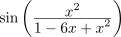 you
simply compute the sine of
rat.
sin(rat)
UnivariatePuiseuxSeries(Expression(Integer), x, 0)
Warning: the type of the coefficients of a power series may affect the kind of computations that you can do with that series. This can only happen when you have made a declaration to specify a series domain with a certain type of coefficient.
If you evaluate then you have declared that y is a one variable Taylor series (UTS is the abbreviation for
UnivariateTaylorSeries) in the variable y with FRAC INT (that is, fractions of integer) coefficients,
centered about 0.
y : UTS(FRAC INT,y,0) := y
UnivariateTaylorSeries(Fraction(Integer), y, 0) You can now compute certain power series in y, provided that these series
have rational coefficients.
exp(y)
UnivariateTaylorSeries(Fraction(Integer), y, 0) You can get examples of such series by applying transcendental functions to
series in y that have no constant terms.
tan(y^2)
UnivariateTaylorSeries(Fraction(Integer), y, 0)
cos(y + y^5)
UnivariateTaylorSeries(Fraction(Integer), y, 0) Similarly, you can compute the logarithm of a power series with rational
coefficients if the constant coefficient is 1.
log(1 + sin(y))
UnivariateTaylorSeries(Fraction(Integer), y, 0) If you wanted to apply, say, the operation exp to a power series with
a nonzero constant coefficient  , then the constant coefficient of the result would be
 ,
which is not a rational number. Therefore, evaluating
exp(2 + tan(y)) would generate an error
message.
If you want to compute the Taylor expansion of exp(2 + tan(y)), you must ensure that the coefficient domain
has an operation exp defined for it. An example of such a domain is Expression Integer, the
type of formal functional expressions over the integers. When working with coefficients of this
type,
z : UTS(EXPR INT,z,0) := z
UnivariateTaylorSeries(Expression(Integer), z, 0) this presents no problems.
exp(2 + tan(z))
UnivariateTaylorSeries(Expression(Integer), z, 0) Another way to create Taylor series whose coefficients are expressions over
the integers is to use taylor which works similarly to series. This is equivalent to the previous computation,
except that now we are using the variable w instead of z.
w := taylor ’w
UnivariateTaylorSeries(Expression(Integer), w, 0)
exp(2 + tan(w))
UnivariateTaylorSeries(Expression(Integer), w, 0)
The ExpressionToUnivariatePowerSeries package provides operations for computing series expansions of functions.
Evaluate this to compute the Taylor expansion of sin x about x = 0. The first argument, sin(x), specifies the
function whose series expansion is to be computed and the second argument, x = 0, specifies that the series is to
be expanded in powers of (x - 0), that is, in powers of x.
taylor(sin(x),x = 0)
UnivariateTaylorSeries(Expression(Integer), x, 0) Here is the Taylor expansion of sin x about  :
taylor(sin(x),x = %pi/6)
UnivariateTaylorSeries(Expression(Integer), x, \%pi/6)
The function to be expanded into a series may have variables other than the series variable. For example, we
may expand tan(x*y) as a Taylor series in x
taylor(tan(x*y),x = 0)
UnivariateTaylorSeries(Expression(Integer), x, 0) or as a Taylor series in y.
taylor(tan(x*y),y = 0)
UnivariateTaylorSeries(Expression(Integer), y, 0) A more interesting function is  .
When we expand this function as a Taylor series in t the  order coefficient is the
 Bernoulli
polynomial divided by
n!.
bern := taylor(t*exp(x*t)/(exp(t) - 1),t = 0)
UnivariateTaylorSeries(Expression(Integer), t, 0) Therefore, this and the next expression produce the same result.
factorial(6) * coefficient(bern,6)
bernoulliB(6,x)
Technically, a series with terms of negative degree is not considered to be a Taylor series, but, rather, a
Laurent series. If you try to compute a Taylor series expansion of  at
x = 1 via taylor(x/log(x),x = 1)
you get an error message. The reason is that the function has a pole at x = 1, meaning that its
series expansion about this point has terms of negative degree. A series with finitely many terms
of negative degree is called a Laurent series. You get the desired series expansion by issuing
this.
laurent(x/log(x),x = 1)
UnivariateLaurentSeries(Expression(Integer), x, 1)
Similarly, a series with terms of fractional degree is neither a Taylor series nor a Laurent series. Such a series
is called a Puiseux series. The expression laurent(sqrt(sec(x)),x = 3 * %pi/2) results in an error message
because the series expansion about this point has terms of fractional degree. However, this command
produces what you want.
puiseux(sqrt(sec(x)),x = 3 * %pi/2)
UnivariatePuiseuxSeries(Expression(Integer), x, (3*\%pi)/2)
Finally, consider the case of functions that do not have Puiseux expansions about certain points. An example
of this is  about
x = 0. puiseux(x^x,x=0) produces an error message because of the type of
singularity of the function at x = 0. The general function series can be used in this case. Notice
that the series returned is not, strictly speaking, a power series because of the log(x) in the
expansion.
series(x^x,x=0)
GeneralUnivariatePowerSeries(Expression(Integer), x, 0)
The GenerateUnivariatePowerSeries package enables you to create power series from explicit formulas for
their  coefficients. In what follows, we construct series expansions for certain transcendental functions by
giving formulas for their coefficients. You can also compute such series expansions directly simply by
specifying the function and the point about which the series is to be expanded. See Section 8.9.5 on page 563
for more information.
Consider the Taylor expansion of  about
x = 0:
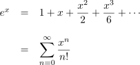
The  Taylor coefficient is
1/n!. This is how you create this series in FriCAS.
series(n +-> 1/factorial(n),x = 0)
UnivariatePuiseuxSeries(Expression(Integer), x, 0)
The first argument specifies a formula for the  coefficient by giving a function that maps
n to 1/n!. The
second argument specifies that the series is to be expanded in powers of (x - 0), that is, in powers of x. Since
we did not specify an initial degree, the first term in the series was the term of degree 0 (the constant term).
Note that the formula was given as an anonymous function. These are discussed in Section 6.17 on page
357.
Consider the Taylor expansion of log x about x = 1:
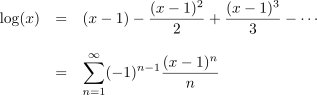
If you were to evaluate the expression series(n you would get an error message
because FriCAS would try to calculate a term of degree  (-1)^(n-1)/ n, x = 1)
0 and therefore divide by 0.
Instead, evaluate this. The third argument, 1.., indicates that only terms of degree n = 1, ... are to be
computed.
series(n +-> (-1)^(n-1)/n,x = 1,1..)
UnivariatePuiseuxSeries(Expression(Integer), x, 1)
Next consider the Taylor expansion of an odd function, say, sin(x):

Here every other coefficient is zero and we would like to give an explicit formula only for the odd Taylor
coefficients. This is one way to do it. The third argument, 1.., specifies that the first term to be computed
is the term of degree 1. The fourth argument, 2, specifies that we increment by 2 to find the
degrees of subsequent terms, that is, the next term is of degree 1 + 2, the next of degree 1 + 2 + 2,
etc.
series(n +-> (-1)^((n-1)/2)/factorial(n),x = 0,1..,2)
UnivariatePuiseuxSeries(Expression(Integer), x, 0)
The initial degree and the increment do not have to be integers. For example, this expression produces a series
expansion of  .
series(n +-> (-1)^((3*n-1)/2)/factorial(3*n),x = 0,1/3..,2/3)
UnivariatePuiseuxSeries(Expression(Integer), x, 0) While the increment must be positive, the initial degree may be negative.
This yields the Laurent expansion of csc(x) at x = 0.
cscx := series(n +-> (-1)^((n-1)/2) * 2 * (2^n-1) * bernoulli(numer(n+1)) / factorial(n+1), x=0, -1..,2)
UnivariatePuiseuxSeries(Expression(Integer), x, 0) Of course, the reciprocal of this power series is the Taylor expansion of
sin(x).
1/cscx
UnivariatePuiseuxSeries(Expression(Integer), x, 0) As a final example, here is the Taylor expansion of asin(x) about
x = 0.
asinx := series(n +-> binomial(n-1,(n-1)/2)/(n*2^(n-1)),x=0,1..,2)
UnivariatePuiseuxSeries(Expression(Integer), x, 0) When we compute the sin of this series, we get x (in the sense that all
higher terms computed so far are zero).
sin(asinx)
UnivariatePuiseuxSeries(Expression(Integer), x, 0)
As we discussed in Section 8.9.5 on page 563, you can also use the operations taylor, laurent and puiseux instead of series if you know ahead of time what kind of exponents a series has. You can’t go wrong using series, though.
Use eval to substitute a numerical value for a variable in a power series. For example, here’s a way to obtain
numerical approximations of %e from the Taylor series expansion of exp(x).
First you create the desired Taylor expansion.
f := taylor(exp(x))
UnivariateTaylorSeries(Expression(Integer), x, 0) Then you evaluate the series at the value 1.0. The result is a sequence of
the partial sums.
eval(f,1.0)
FriCAS provides operations for computing definite and indefinite sums.
You can compute the sum of the first ten fourth powers by evaluating this. This creates a list whose
entries are  as
 ranges from 1 to 10, and then computes the sum of the entries of that
list.
reduce(+,[m^4 for m in 1..10])
PositiveInteger You can also compute a formula for the sum of the first  fourth powers, where
 is an
unspecified positive integer.
sum4 := sum(m^4, m = 1..k)
Fraction(Polynomial(Integer)) This formula is valid for any positive integer  . For instance, if we replace
 by 10, we
obtain the number we computed earlier.
eval(sum4, k = 10)
You can compute a formula for the sum of the first 
 powers in a similar fashion. Just replace the
4 in
the definition of sum4 by any expression not involving  . FriCAS computes these formulas using Bernoulli
polynomials; we use the rest of this section to describe this method.
First consider this function of t and x.
f := t*exp(x*t) / (exp(t) - 1)
Expression(Integer) Since the expressions involved get quite large, we tell FriCAS to show us only terms of
degree up to 5.
)set streams calculate 5
If we look at the Taylor expansion of f(x, t) about t = 0, we see that the coefficients of the powers of t are
polynomials in x.
ff := taylor(f,t = 0)
UnivariateTaylorSeries(Expression(Integer), t, 0) In fact, the  coefficient in this series is essentially the
 Bernoulli
polynomial: the
 coefficient of the series is
 , where
 is the
 Bernoulli polynomial.
Thus, to obtain the
 Bernoulli polynomial, we multiply the
 coefficient of the series
ff by n!. For
example, the sixth Bernoulli polynomial is this.
factorial(6) * coefficient(ff,6)
Expression(Integer) We derive some properties of the function f(x,t). First we compute
f(x + 1,t)- f(x,t).
g := eval(f, x = x + 1) - f
Expression(Integer) If we normalize g, we see that it has a particularly simple form.
normalize(g)
Expression(Integer) From this it follows that the  coefficient in the Taylor expansion of
g(x,t) at t = 0 is
 . If you want to check this, evaluate the next expression.
taylor(g,t = 0)
UnivariateTaylorSeries(Expression(Integer), t, 0) However, since g(x,t)= f(x+1,t)-f(x,t), it follows that the  coefficient
is
 . Equating coefficients, we see that
 and,
therefore,
 . Let’s apply this formula repeatedly, letting
x vary between two
integers a and b, with a < b:
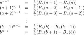
When we add these equations we find that the sum of the left-hand sides is  the sum of the
 powers from
a to b. The sum of the right-hand sides is a “telescoping series.” After cancellation,
the sum is simply  .
Replacing n by n + 1, we have shown that

Let’s use this to obtain the formula for the sum of fourth powers. First we obtain the Bernoulli polynomial
 .
B5 := factorial(5) * coefficient(ff,5)
Expression(Integer) To find the sum of the first  4th powers, we multiply
1/5 by  .
1/5 * (eval(B5, x = k + 1) - eval(B5, x = 1))
Expression(Integer) This is the same formula that we obtained via sum(m^4, m = 1..k).
sum4
At this point you may want to do the same computation, but with an exponent other than 4. For example,
you might try to find a formula for the sum of the first  20th powers.
In this section we discuss FriCAS’s facilities for solving differential equations in closed-form and in series.
FriCAS provides facilities for closed-form solution of single differential equations of the following kinds:
For a discussion of the solution of systems of linear and polynomial equations, see Section 8.5 on page 521.
A differential equation is an equation involving an unknown function and one or more of its derivatives. The equation is called ordinary if derivatives with respect to only one dependent variable appear in the equation (it is called partial otherwise). The package ElementaryFunctionODESolver provides the top-level operation solve for finding closed-form solutions of ordinary differential equations.
To solve a differential equation, you must first create an operator for the unknown function. We let y be the
unknown function in terms of x.
y := operator ’y
BasicOperator You then type the equation using D to create the derivatives of the unknown function y(x) where x
is any symbol you choose (the so-called dependent variable). This is how you enter the equation
y’’ + y’ + y = 0.
deq := D(y x, x, 2) + D(y x, x) + y x = 0
Equation(Expression(Integer)) The simplest way to invoke the solve command is with three arguments.
So, to solve the above equation, we enter this.
solve(deq, y, x)
Union(Record(particular: Expression(Integer), basis: List(Expression(Integer))), ...) Since linear ordinary differential equations have infinitely many solutions, solve returns a
particular solution  and a basis
 for the solutions of the corresponding homogeneous equation.
Any expression of the form
 where the
 do not involve the dependent variable
is also a solution. This is similar to what you get when you solve systems of linear algebraic
equations.
A way to select a unique solution is to specify initial conditions: choose a value a for the dependent variable
and specify the values of the unknown function and its derivatives at a. If the number of initial conditions is
equal to the order of the equation, then the solution is unique (if it exists in closed form!) and solve tries to
find it. To specify initial conditions to solve, use an Equation of the form x = a for the third parameter
instead of the dependent variable, and add a fourth parameter consisting of the list of values
y(a), y’(a), ....
To find the solution of y’’ + y = 0 satisfying y(0)= y’(0)= 1, do this.
deq := D(y x, x, 2) + y x
Expression(Integer) You can omit the = 0 when you enter the equation to be solved.
solve(deq, y, x = 0, [1, 1])
Union(Expression(Integer), ...)
FriCAS is not limited to linear differential equations with constant coefficients. It can also find solutions when the coefficients are rational or algebraic functions of the dependent variable. Furthermore, FriCAS is not limited by the order of the equation. FriCAS can solve the following third order equations with polynomial coefficients.
deq := x^3 * D(y x, x, 3) + x^2 * D(y x, x, 2) - 2 * x * D(y x, x) + 2 * y x = 2 * x^4
solve(deq, y, x)
Union(Record(particular: Expression(Integer), basis: List(Expression(Integer))), ...) Here we are solving a homogeneous equation.
deq := (x^9+x^3) * D(y x, x, 3) + 18 * x^8 * D(y x, x, 2) - 90 * x * D(y x, x) - 30 * (11 * x^6 - 3) * y x
solve(deq, y, x)
Union(Record(particular: Expression(Integer), basis: List(Expression(Integer))), ...) On the other hand, and in contrast with the operation integrate, it can happen that FriCAS finds no solution and that some closed-form solution still exists. While it is mathematically complicated to describe exactly when the solutions are guaranteed to be found, the following statements are correct and form good guidelines for linear ordinary differential equations:
Note that this last statement does not mean that FriCAS does not find the solutions that are algebraic functions. It means that it is not guaranteed that the algebraic function solutions will be found. This is an example where all the algebraic solutions are found.
deq := (x^2 + 1) * D(y x, x, 2) + 3 * x * D(y x, x) + y x = 0
solve(deq, y, x)
Union(Record(particular: Expression(Integer), basis: List(Expression(Integer))), ...)
This is an example that shows how to solve a non-linear first order ordinary differential equation manually when an integrating factor can be found just by integration. At the end, we show you how to solve it directly.
Let’s solve the differential equation y’ = y / (x + y log y). Using the notation m(x, y)+ n(x, y)y’ = 0, we have m = -y
and n = x + y log y.
m := -y
n := x + y * log y
Expression(Integer) We first check for exactness, that is, does dm/dy = dn/dx?
D(m, y) - D(n, x)
Expression(Integer) This is not zero, so the equation is not exact. Therefore we must look for
an integrating factor: a function  (x,y)
d(. Normally, we
first search for  m)/dy = d(
 n)/dx
 (x,y)
x or only on y. Let’s search for such a  (x)
mu := operator ’mu
a := D(mu(x) * m, y) - D(mu(x) * n, x)
Expression(Integer) If the above is zero for a function 
y, then  (x)
solve(a = 0, mu, x)
Union(Record(particular: Expression(Integer), basis: List(Expression(Integer))), ...) The solution depends on y, so there is no integrating factor that depends on x only. Let’s
look for one that depends on y only.
b := D(mu(y) * m, y) - D(mu(y) * n, x)
sb := solve(b = 0, mu, y)
Union(Record(particular: Expression(Integer), basis: List(Expression(Integer))), ...) We’ve found one! The above  (y)
m and n) by the integrating factor.
intFactor := sb.basis.1
m := intFactor * m
n := intFactor * n
Expression(Integer) Let’s check for exactness.
D(m, y) - D(n, x)
Expression(Integer) We must solve the exact equation, that is, find a function s(x,y) such that ds/dx = m and
ds/dy = n. We start by writing s(x, y)= h(y)+ integrate(m, x) where h(y) is an unknown function of y. This
guarantees that ds/dx = m.
h := operator ’h
sol := h y + integrate(m, x)
Expression(Integer) All we want is to find h(y) such that ds/dy = n.
dsol := D(sol, y)
nsol := solve(dsol = n, h, y)
Union(Record(particular: Expression(Integer), basis: List(Expression(Integer))), ...) The above particular solution is the h(y) we want, so we just replace h(y) by it in the
implicit solution.
eval(sol, h y = nsol.particular)
Expression(Integer) A first integral of the initial equation is obtained by setting this result equal to an arbitrary constant.
Now that we’ve seen how to solve the equation “by hand,” we show you how to do it with the solve operation.
First define y to be an operator.
y := operator ’y
BasicOperator Next we create the differential equation.
deq := D(y x, x) = y(x) / (x + y(x) * log y x)
Equation(Expression(Integer)) Finally, we solve it.
solve(deq, y, x)
Union(Expression(Integer), ...)
The command to solve differential equations in power series around a particular initial point with specific initial conditions is called seriesSolve. It can take a variety of parameters, so we illustrate its use with some examples.
Since the coefficients of some solutions are quite large, we reset the default to compute only seven terms.
)set streams calculate 7
You can solve a single nonlinear equation of any order. For example, we solve y’’’ = sin(y’’)* exp(y)+ cos(x)
subject to y(0)= 1, y’(0)= 0, y’’(0)= 0.
We first tell FriCAS that the symbol ’y denotes a new operator.
y := operator ’y
BasicOperator Enter the differential equation using y like any system function.
eq := D(y(x), x, 3) - sin(D(y(x), x, 2))*exp(y(x)) = cos(x)
Equation(Expression(Integer)) Solve it around x = 0 with the initial conditions y(0)= 1, y’(0)= y’’(0)= 0.
seriesSolve(eq, y, x = 0, [1, 0, 0])
Compiling function %JJ with type List(UnivariateTaylorSeries(Expression(Integer ),x,0)) -> UnivariateTaylorSeries(Expression(Integer),x,0)
UnivariateTaylorSeries(Expression(Integer), x, 0)
You can also solve a system of nonlinear first order equations. For example, we solve a system that has tan(t)
and sec(t) as solutions.
We tell FriCAS that x is also an operator.
x := operator ’x
Compiled code for %JJ has been cleared.
BasicOperator Enter the two equations forming our system.
eq1 := D(x(t), t) = 1 + x(t)^2
eq2 := D(y(t), t) = x(t) * y(t)
Equation(Expression(Integer)) Solve the system around t = 0 with the initial conditions x(0)= 0 and y(0)= 1. Notice that
since we give the unknowns in the order [x, y], the answer is a list of two series in the order
[series for x(t), series for y(t)].
seriesSolve([eq2, eq1], [x, y], t = 0, [y(0) = 1, x(0) = 0])
Compiling function %JP with type List(UnivariateTaylorSeries(Expression(Integer ),t,0)) -> UnivariateTaylorSeries(Expression(Integer),t,0)
Compiling function %JQ with type List(UnivariateTaylorSeries(Expression(Integer ),t,0)) -> UnivariateTaylorSeries(Expression(Integer),t,0)
List(UnivariateTaylorSeries(Expression(Integer), t, 0)) The order in which we give the equations and the initial conditions has no effect on the order of the solution.
A finite field (also called a Galois field) is a finite algebraic structure where one can add, multiply and divide
under the same laws (for example, commutativity, associativity or distributivity) as apply to the rational,
real or complex numbers. Unlike those three fields, for any finite field there exists a positive
prime integer  , called the characteristic, such that
 for any element
 in the finite
field. In fact, the number of elements in a finite field is a power of the characteristic and for each
prime
 and positive integer
 there exists exactly one finite field with
 elements, up to
isomorphism.1
When n = 1, the field has  elements and is called a prime field, discussed in the next section. There are
several ways of implementing extensions of finite fields, and FriCAS provides quite a bit of freedom to allow
you to choose the one that is best for your application. Moreover, we provide operations for converting
among the different representations of extensions and different extensions of a single field. Finally,
note that you usually need to package-call operations from finite fields if the operations do not
take as an argument an object of the field. See Section 2.9 on page 179 for more information on
package-calling.
Let  be a positive integer. It is well known that you can get the same result if you perform addition,
subtraction or multiplication of integers and then take the remainder on dividing by
 as if you had first
done such remaindering on the operands, performed the arithmetic and then (if necessary) done remaindering
again. This allows us to speak of arithmetic modulo
 or, more simply mod
 . In FriCAS, you use
IntegerMod to do such arithmetic.
(a,b) : IntegerMod 12
(a, b) := (16, 7)
[a - b, a * b]
List(IntegerMod(12)) If  is not prime, there is only a limited notion of reciprocals and division.
a / b
There are 10 exposed and 16 unexposed library operations named / having 2 argument(s) but none was determined to be applicable. Use HyperDoc Browse, or issue )display op / to learn more about the available operations. Perhaps package-calling the operation or using coercions on the arguments will allow you to apply the operation.
Cannot find a definition or applicable library operation named / with argument type(s) IntegerMod(12) IntegerMod(12) Perhaps you should use "@" to indicate the required return type, or "$" to specify which version of the function you need.
recip a
Union("failed", ...) Here 7 and 12 are relatively prime, so 7 has a multiplicative inverse modulo
12.
recip b
If we take  to be a prime number
 , then taking inverses and, therefore, division are generally defined.
Use PrimeField instead of IntegerMod for
 prime.
c : PrimeField 11 := 8
inv c
PrimeField(11) You can also use 1/c and c^(-1) for the inverse of  .
9/c
PrimeField (abbreviation PF) checks if its argument is prime when you try to use an operation from it. If you know the argument is prime (particularly if it is large), InnerPrimeField (abbreviation IPF) assumes the argument has already been verified to be prime. If you do use a number that is not prime, you will eventually get an error message, most likely a division by zero message. For computer science applications, the most important finite fields are PrimeField 2 and its extensions.
In the following examples, we work with the finite field with  elements.
GF101 := PF 101
Type Like many domains in FriCAS, finite fields provide an operation for returning a random element of the domain.
x := random()$GF101
y : GF101 := 37
z := x/y
z * y - x
PrimeField(101) The element 2 is a primitive element of this field,
pe := primitiveElement()$GF101
PrimeField(101) in the sense that its powers enumerate all nonzero elements.
[pe^i for i in 0..99]
List(PrimeField(101)) If every nonzero element is a power of a primitive element, how do you determine what the exponent is? Use discreteLog.
ex := discreteLog(y)
pe ^ ex
PrimeField(101) The order of a nonzero element  is the smallest positive integer
 such
 .
order y
PositiveInteger The order of a primitive element is the defining  .
order pe
When you want to work with an extension of a finite field in FriCAS, you have three choices to make:
This illustrates one of the most important features of FriCAS: you can choose exactly the right data-type and representation to suit your application best.
We first tell you what domain constructors to use for each case above, and then give some examples.
Constructors that automatically generate extensions of the prime field:
FiniteField
FiniteFieldCyclicGroup
FiniteFieldNormalBasis
Constructors that generate extensions of an arbitrary field:
FiniteFieldExtension
FiniteFieldExtensionByPolynomial
FiniteFieldCyclicGroupExtension
FiniteFieldCyclicGroupExtensionByPolynomial
FiniteFieldNormalBasisExtension
FiniteFieldNormalBasisExtensionByPolynomial
Constructors that use a cyclic group representation:
FiniteFieldCyclicGroup
FiniteFieldCyclicGroupExtension
FiniteFieldCyclicGroupExtensionByPolynomial
Constructors that use a normal basis representation:
FiniteFieldNormalBasis
FiniteFieldNormalBasisExtension
FiniteFieldNormalBasisExtensionByPolynomial
Constructors that use an irreducible modulus polynomial representation:
FiniteField
FiniteFieldExtension
FiniteFieldExtensionByPolynomial
Constructors that generate a polynomial for you:
FiniteField
FiniteFieldExtension
FiniteFieldCyclicGroup
FiniteFieldCyclicGroupExtension
FiniteFieldNormalBasis
FiniteFieldNormalBasisExtension
Constructors for which you provide a polynomial:
FiniteFieldExtensionByPolynomial
FiniteFieldCyclicGroupExtensionByPolynomial
FiniteFieldNormalBasisExtensionByPolynomial
These constructors are discussed in the following sections where we collect together descriptions of extension fields that have the same underlying representation.2
If you don’t really care about all this detail, just use FiniteField. As your knowledge of your application and its FriCAS implementation grows, you can come back and choose an alternative constructor that may improve the efficiency of your code. Note that the exported operations are almost the same for all constructors of finite field extensions and include the operations exported by PrimeField.
All finite field extension constructors discussed in this section use a representation that performs arithmetic with univariate (one-variable) polynomials modulo an irreducible polynomial. This polynomial may be given explicitly by you or automatically generated. The ground field may be the prime field or one you specify. See Section 8.11.2 on page 607 for general information about finite field extensions.
For FiniteField (abbreviation FF) you provide a prime number  and an extension degree
 . This degree
can be 1. FriCAS uses the prime field PrimeField(p), here PrimeField 2, and it chooses an irreducible
polynomial of degree
 , here 12, over the ground field.
GF4096 := FF(2,12);
The objects in the generated field extension are polynomials of degree at most  with coefficients in the
prime field. The polynomial indeterminate is automatically chosen by FriCAS and is typically something like
%A or %D. These (strange) variables are only for output display; there are several ways to construct elements of
this field.
The operation index enumerates the elements of the field extension and accepts as argument the integers from
1 to  . The expression
index(p) always gives the indeterminate.
a := index(2)$GF4096
FiniteField(2, 12) You can build polynomials in  and calculate in
GF4096.
b := a^12 - a^5 + a
b ^ 1000
c := a/b
FiniteField(2, 12) Among the available operations are norm and trace.
norm c
trace c
Since any nonzero element is a power of a primitive element, how do we discover what the exponent is? The operation discreteLog calculates the exponent and, if it is called with only one argument, always refers to the primitive element returned by primitiveElement.
dL := discreteLog a
g ^ dL
FiniteFieldExtension (abbreviation FFX) is similar to FiniteField except that the ground-field for FiniteFieldExtension is arbitrary and chosen by you. In case you select the prime field as ground field, there is essentially no difference between the constructed two finite field extensions.
GF16 := FF(2,4);
GF4096 := FFX(GF16,3);
r := (random()$GF4096) ^ 20
FiniteFieldExtension(FiniteField(2, 4), 3)
norm(r)
FiniteFieldExtensionByPolynomial (abbreviation FFP) is similar to FiniteField and FiniteFieldExtension but is more general.
GF4 := FF(2,2);
f := nextIrreduciblePoly(random(6)$FFPOLY(GF4))$FFPOLY(GF4)
Union(SparseUnivariatePolynomial(FiniteField(2, 2)), ...) For FFP you choose both the ground field and the irreducible polynomial used in the representation. The degree of the extension is the degree of the polynomial.
GF4096 := FFP(GF4,f);
discreteLog random()$GF4096
In every finite field there exist elements whose powers are all the nonzero elements of the field. Such an element is called a primitive element.
In FiniteFieldCyclicGroup (abbreviation FFCG) the nonzero elements are represented by the powers of a fixed primitive element of the field (that is, a generator of its cyclic multiplicative group). Multiplication (and hence exponentiation) using this representation is easy. To do addition, we consider our primitive element as the root of a primitive polynomial (an irreducible polynomial whose roots are all primitive). See Section 8.11.7 on page 631 for examples of how to compute such a polynomial.
To use FiniteFieldCyclicGroup you provide a prime number and an extension degree.
GF81 := FFCG(3,4);
Type FriCAS uses the prime field, here PrimeField 3, as the ground field and it chooses a primitive
polynomial of degree  , here 4, over the prime field.
a := primitiveElement()$GF81
FiniteFieldCyclicGroup(3, 4) You can calculate in GF81.
b := a^12 - a^5 + a
FiniteFieldCyclicGroup(3, 4) In this representation of finite fields the discrete logarithm of an element can be seen directly in its output form.
b
discreteLog b
FiniteFieldCyclicGroupExtension (abbreviation FFCGX) is similar to FiniteFieldCyclicGroup except that the ground field for FiniteFieldCyclicGroupExtension is arbitrary and chosen by you. In case you select the prime field as ground field, there is essentially no difference between the constructed two finite field extensions.
GF9 := FF(3,2);
GF729 := FFCGX(GF9,3);
r := (random()$GF729) ^ 20
FiniteFieldCyclicGroupExtension(FiniteField(3, 2), 3)
trace(r)
FiniteFieldCyclicGroupExtensionByPolynomial (abbreviation FFCGP) is similar to FiniteFieldCyclicGroup and FiniteFieldCyclicGroupExtension but is more general. For FiniteFieldCyclicGroupExtensionByPolynomial you choose both the ground field and the irreducible polynomial used in the representation. The degree of the extension is the degree of the polynomial.
GF3 := PrimeField 3;
Type We use a utility operation to generate an irreducible primitive polynomial (see Section 8.11.7 on page 631). The polynomial has one variable that is “anonymous”: it displays as a question mark.
f := createPrimitivePoly(4)$FFPOLY(GF3)
SparseUnivariatePolynomial(PrimeField(3))
GF81 := FFCGP(GF3,f);
Type Let’s look at a random element from this field.
random()$GF81
FiniteFieldCyclicGroupExtensionByPolynomial(PrimeField(3), ?^4+?+2)
Let  be a finite extension of degree
 of the finite field
 and let
 have
 elements. An element
 of
 is said to be normal over
 if the elements

form a basis of  as a vector space over
 . Such a basis is called a normal
basis.3
If  is normal over
 , its minimal polynomial is also said to be normal over
 . There exist normal bases
for all finite extensions of arbitrary finite fields.
In FiniteFieldNormalBasis (abbreviation FFNB), the elements of the finite field are represented by coordinate vectors with respect to a normal basis.
You provide a prime  and an extension degree
 .
K := FFNB(3,8)
Type FriCAS uses the prime field PrimeField(p), here PrimeField 3, and it chooses a normal
polynomial of degree  , here 8, over the ground field. The remainder class of the indeterminate is used as
the normal element. The polynomial indeterminate is automatically chosen by FriCAS and is
typically something like
%A or %D. These (strange) variables are only for output display; there are
several ways to construct elements of this field. The output of the basis elements is something like
 .
a := normalElement()$K
FiniteFieldNormalBasis(3, 8) You can calculate in  using
 .
b := a^12 - a^5 + a
FiniteFieldNormalBasisExtension (abbreviation FFNBX) is similar to FiniteFieldNormalBasis except that the groundfield for FiniteFieldNormalBasisExtension is arbitrary and chosen by you. In case you select the prime field as ground field, there is essentially no difference between the constructed two finite field extensions.
GF9 := FFNB(3,2);
GF729 := FFNBX(GF9,3);
r := random()$GF729
FiniteFieldNormalBasisExtension(FiniteFieldNormalBasis(3, 2), 3)
r + r^3 + r^9 + r^27
FiniteFieldNormalBasisExtension(FiniteFieldNormalBasis(3, 2), 3)
FiniteFieldNormalBasisExtensionByPolynomial (abbreviation FFNBP) is similar to FiniteFieldNormalBasis and FiniteFieldNormalBasisExtension but is more general. For FiniteFieldNormalBasisExtensionByPolynomial you choose both the ground field and the irreducible polynomial used in the representation. The degree of the extension is the degree of the polynomial.
GF3 := PrimeField 3;
Type We use a utility operation to generate an irreducible normal polynomial (see Section 8.11.7 on page 631). The polynomial has one variable that is “anonymous”: it displays as a question mark.
f := createNormalPoly(4)$FFPOLY(GF3)
SparseUnivariatePolynomial(PrimeField(3))
GF81 := FFNBP(GF3,f);
Type Let’s look at a random element from this field.
r := random()$GF81
FiniteFieldNormalBasisExtensionByPolynomial(PrimeField(3), ?^4+2*?^3+2)
r * r^3 * r^9 * r^27
FiniteFieldNormalBasisExtensionByPolynomial(PrimeField(3), ?^4+2*?^3+2)
norm r
Let  be a finite field.
K := PrimeField 3
Type An extension field  of degree
 over
 is a subfield of an extension field
 of degree
 over
 if and only if
 divides
 .
 |
||
 |
||
 |  |  |
 |
||
| K |
FiniteFieldHomomorphisms provides conversion operations between different extensions of one fixed finite
ground field and between different representations of these finite fields. Let’s choose  and
 ,
(m,n) := (4,8)
PositiveInteger build the field extensions,
Km := FiniteFieldExtension(K,m)
Type and pick two random elements from the smaller field.
Kn := FiniteFieldExtension(K,n)
a1 := random()$Km
FiniteFieldExtension(PrimeField(3), 4)
b1 := random()$Km
FiniteFieldExtension(PrimeField(3), 4) Since  divides
 ,
 is a subfield of
 .
a2 := a1 :: Kn
FiniteFieldExtension(PrimeField(3), 8) Therefore we can convert the elements of  into elements of
 .
b2 := b1 :: Kn
FiniteFieldExtension(PrimeField(3), 8) To check this, let’s do some arithmetic.
a1+b1 - ((a2+b2) :: Km)
FiniteFieldExtension(PrimeField(3), 4)
a1*b1 - ((a2*b2) :: Km)
FiniteFieldExtension(PrimeField(3), 4) There are also conversions available for the situation, when  and
 are
represented in different ways (see Section 8.11.2 on page 607). For example let’s choose
 where the representation is 0 plus the cyclic multiplicative group and
 with a normal basis
representation.
Km := FFCGX(K,m)
Kn := FFNBX(K,n)
(a1,b1) := (random()$Km,random()$Km)
FiniteFieldCyclicGroupExtension(PrimeField(3), 4)
a2 := a1 :: Kn
FiniteFieldNormalBasisExtension(PrimeField(3), 8)
b2 := b1 :: Kn
FiniteFieldNormalBasisExtension(PrimeField(3), 8) Check the arithmetic again.
a1+b1 - ((a2+b2) :: Km)
FiniteFieldCyclicGroupExtension(PrimeField(3), 4)
a1*b1 - ((a2*b2) :: Km)
FiniteFieldCyclicGroupExtension(PrimeField(3), 4)
FiniteFieldPolynomialPackage (abbreviation FFPOLY) provides operations for generating, counting and testing polynomials over finite fields. Let’s start with a couple of definitions:
In what follows, many of the generated polynomials have one “anonymous” variable. This indeterminate is displayed as a question mark (“?”).
To fix ideas, let’s use the field with five elements for the first few examples.
GF5 := PF 5;
Type You can generate irreducible polynomials of any (positive) degree (within the storage capabilities of the computer and your ability to wait) by using createIrreduciblePoly.
f := createIrreduciblePoly(8)$FFPOLY(GF5)
SparseUnivariatePolynomial(PrimeField(5)) Does this polynomial have other important properties? Use primitive? to test whether it is a primitive polynomial.
primitive?(f)$FFPOLY(GF5)
Boolean Use normal? to test whether it is a normal polynomial.
normal?(f)$FFPOLY(GF5)
Boolean Note that this is actually a trivial case, because a normal polynomial of degree  must have a
nonzero term of degree
 . We will refer back to this later.
To get a primitive polynomial of degree 8 just issue this.
p := createPrimitivePoly(8)$FFPOLY(GF5)
SparseUnivariatePolynomial(PrimeField(5))
primitive?(p)$FFPOLY(GF5)
Boolean This polynomial is not normal,
normal?(p)$FFPOLY(GF5)
Boolean but if you want a normal one simply write this.
n := createNormalPoly(8)$FFPOLY(GF5)
SparseUnivariatePolynomial(PrimeField(5)) This polynomial is not primitive!
primitive?(n)$FFPOLY(GF5)
Boolean This could have been seen directly, as the constant term is 1 here,
which is not a primitive element up to the factor (-1) raised to the degree of the
polynomial.4
What about polynomials that are both primitive and normal? The existence of such a polynomial is by no means obvious. 5 If you really need one use either createPrimitiveNormalPoly or createNormalPrimitivePoly.
createPrimitiveNormalPoly(8)$FFPOLY(GF5)
SparseUnivariatePolynomial(PrimeField(5))
If you want to obtain additional polynomials of the various types above as given by the create... operations above, you can use the next... operations. For instance, nextIrreduciblePoly yields the next monic irreducible polynomial with the same degree as the input polynomial. By “next” we mean “next in a natural order using the terms and coefficients.” This will become more clear in the following examples.
This is the field with five elements.
GF5 := PF 5;
Type Our first example irreducible polynomial, say of degree 3, must be “greater” than this.
h := monomial(1,8)$SUP(GF5)
SparseUnivariatePolynomial(PrimeField(5)) You can generate it by doing this.
nh := nextIrreduciblePoly(h)$FFPOLY(GF5)
Union(SparseUnivariatePolynomial(PrimeField(5)), ...) Notice that this polynomial is not the same as the one createIrreduciblePoly.
createIrreduciblePoly(3)$FFPOLY(GF5)
SparseUnivariatePolynomial(PrimeField(5)) You can step through all irreducible polynomials of degree 8 over the field with 5 elements by repeatedly issuing this.
nh := nextIrreduciblePoly(nh)$FFPOLY(GF5)
Union(SparseUnivariatePolynomial(PrimeField(5)), ...) You could also ask for the total number of these.
numberOfIrreduciblePoly(5)$FFPOLY(GF5)
We hope that “natural order” on polynomials is now clear: first we compare the number of monomials of two polynomials (“more” is “greater”); then, if necessary, the degrees of these monomials (lexicographically), and lastly their coefficients (also lexicographically, and using the operation lookup if our field is not a prime field). Also note that we make both polynomials monic before looking at the coefficients: multiplying either polynomial by a nonzero constant produces the same result.
The package FiniteFieldPolynomialPackage also provides similar operations for primitive and normal polynomials. With the exception of the number of primitive normal polynomials; we’re not aware of any known formula for this.
numberOfPrimitivePoly(3)$FFPOLY(GF5)
PositiveInteger Take these,
m := monomial(1,1)$SUP(GF5)
SparseUnivariatePolynomial(PrimeField(5))
f := m^3 + 4*m^2 + m + 2
SparseUnivariatePolynomial(PrimeField(5)) and then we have:
f1 := nextPrimitivePoly(f)$FFPOLY(GF5)
Union(SparseUnivariatePolynomial(PrimeField(5)), ...) What happened?
nextPrimitivePoly(f1)$FFPOLY(GF5)
Union(SparseUnivariatePolynomial(PrimeField(5)), ...) Well, for the ordering used in nextPrimitivePoly we use as first criterion a comparison of the constant terms of the polynomials. Analogously, in nextNormalPoly we first compare the monomials of degree 1 less than the degree of the polynomials (which is nonzero, by an earlier remark).
f := m^3 + m^2 + 4*m + 1
SparseUnivariatePolynomial(PrimeField(5))
f1 := nextNormalPoly(f)$FFPOLY(GF5)
Union(SparseUnivariatePolynomial(PrimeField(5)), ...)
nextNormalPoly(f1)$FFPOLY(GF5)
Union(SparseUnivariatePolynomial(PrimeField(5)), ...) We don’t have to restrict ourselves to prime fields. Let’s consider, say, a field with 16 elements.
GF16 := FFX(FFX(PF 2,2),2);
Type We can apply any of the operations described above.
createIrreduciblePoly(5)$FFPOLY(GF16)
SparseUnivariatePolynomial(FiniteFieldExtension(FiniteFieldExtension(PrimeField(2), 2), 2))
FriCAS also provides operations for producing random polynomials of a given degree
random(5)$FFPOLY(GF16)
SparseUnivariatePolynomial(FiniteFieldExtension(FiniteFieldExtension(PrimeField(2), 2), 2)) or with degree between two given bounds.
random(3,9)$FFPOLY(GF16)
SparseUnivariatePolynomial(FiniteFieldExtension(FiniteFieldExtension(PrimeField(2), 2), 2))
FiniteFieldPolynomialPackage2 (abbreviation FFPOLY2) exports an operation rootOfIrreduciblePoly for
finding one root of an irreducible polynomial f in an extension field of the coefficient field. The degree of
the extension has to be a multiple of the degree of f. It is not checked whether f actually is
irreducible.
To illustrate this operation, we fix a ground field GF
GF2 := PrimeField 2;
Type and then an extension field.
F := FFX(GF2,12)
Type We construct an irreducible polynomial over GF2.
f := createIrreduciblePoly(6)$FFPOLY(GF2)
SparseUnivariatePolynomial(PrimeField(2)) We compute a root of f.
root := rootOfIrreduciblePoly(f)$FFPOLY2(F,GF2)
FiniteFieldExtension(PrimeField(2), 12)
FriCAS provides a facility for the primary decomposition of polynomial ideals over fields of characteristic zero. The algorithm works in essentially two steps:
The FriCAS constructor PolynomialIdeal represents ideals with coefficients in any field and supports the basic ideal operations, including intersection, sum and quotient. IdealDecompositionPackage contains the specific operations for the primary decomposition and the computation of the radical of an ideal with polynomial coefficients in a field of characteristic 0 with an effective algorithm for factoring polynomials.
The following examples illustrate the capabilities of this facility. First consider the ideal generated by
 (which defines a circle in the
(x,y)-plane) and the ideal generated by  (corresponding
to the straight lines
x = y and x = -y.
(n,m) : List DMP([x,y],FRAC INT)
m := [x^2+y^2-1]
List(DistributedMultivariatePolynomial([x, y], Fraction(Integer)))
n := [x^2-y^2]
List(DistributedMultivariatePolynomial([x, y], Fraction(Integer))) We find the equations defining the intersection of the two loci. This correspond to the sum of the associated ideals.
id := ideal m + ideal n
PolynomialIdeal(Fraction(Integer), DirectProduct(2, NonNegativeInteger), OrderedVariableList([x, y]), DistributedMultivariatePolynomial([x, y], Fraction(Integer))) We can check if the locus contains only a finite number of points, that is, if the ideal is zero-dimensional.
zeroDim? id
zeroDim?(ideal m)
dimension ideal m
PositiveInteger We can find polynomial relations among the generators (f and g are the parametric equations of
the knot).
(f,g):DMP([x,y],FRAC INT)
f := x^2-1
DistributedMultivariatePolynomial([x, y], Fraction(Integer))
g := x*(x^2-1)
DistributedMultivariatePolynomial([x, y], Fraction(Integer))
relationsIdeal [f,g]
SuchThat(List(Polynomial(Fraction(Integer))), List(Equation(Polynomial(Fraction(Integer)))))
We can compute the primary decomposition of an ideal.
l: List DMP([x,y,z],FRAC INT) := [x^2+2*y^2,x*z^2-y*z,z^2-4]
List(DistributedMultivariatePolynomial([x, y, z], Fraction(Integer)))
ld:=primaryDecomp(ideal l)$IdealDecompositionPackage([x,y,z])
List(PolynomialIdeal(Fraction(Integer), DirectProduct(3, NonNegativeInteger), OrderedVariableList([x, y, z]), DistributedMultivariatePolynomial([x, y, z], Fraction(Integer)))) We can intersect back.
reduce(intersect,ld)
We can compute the radical of every primary component.
reduce(intersect,[radical(ld.i)$IdealDecompositionPackage([x,y,z]) for i in 1..2])
PolynomialIdeal(Fraction(Integer), DirectProduct(3, NonNegativeInteger), OrderedVariableList([x, y, z]), DistributedMultivariatePolynomial([x, y, z], Fraction(Integer))) Their intersection is equal to the radical of the ideal of l.
radical(ideal l)$IdealDecompositionPackage([x,y,z])
As a sample use of FriCAS’s algebraic number facilities, we compute the Galois group of the polynomial
 .
p := x^5 - 5*x + 12
Polynomial(Integer) We would like to construct a polynomial  such that the splitting field of
 is
generated by one root of
 . First we construct a polynomial
 such that one root of
 generates the field generated by two roots of the polynomial
 . (As it will turn out, the field generated by
two roots of
 is, in fact, the splitting field of
 .)
From the proof of the primitive element theorem we know that if  and
 are algebraic numbers, then the
field
 is equal to
 for an appropriately chosen integer
 . In our case, we construct the
minimal polynomial of
 , where
 and
 are two roots of
 . We construct this polynomial
using resultant. The main result we need is the following: If
 is a polynomial with roots
 and
 is a polynomial with roots
 , then the polynomial
h(x)= resultant(f(y), g(x-y), y) is a
polynomial of degree  with roots
 .
For  we use the polynomial
 . For
 we use the polynomial
 . Thus, the polynomial
we first construct is
resultant(p(y), -p(y-x), y).
q := resultant(eval(p,x,y),-eval(p,x,y-x),y)
Polynomial(Integer) The roots of  are
 . Of course, there are five pairs
 with
 , so
0 is a 5-fold root of  . Let’s get rid of this factor.
q1 := exquo(q, x^5)
Union(Polynomial(Integer), ...) Factor the polynomial q1.
factoredQ := factor q1
Factored(Polynomial(Integer)) We see that q1 has two irreducible factors, each of degree 10. (The fact that the polynomial q1
has two factors of degree 10 is enough to show that the Galois group of  is the dihedral group of order
10.6
Note that the type of factoredQ is FR POLY INT, that is, Factored Polynomial Integer. This is a
special data type for recording factorizations of polynomials with integer coefficients (see ‘Factored’ on page
857). We can access the individual factors using the operation factorList.
r := factorList(factoredQ).1.factor
Consider the polynomial  . This is the minimal polynomial of the difference of two roots of
 .
Thus, the splitting field of
 contains a subfield of degree
10. We show that this subfield is, in fact, the
splitting field of  by showing that
 factors completely over this field. First we create a symbolic
root of the polynomial
 . (We replaced
x by b in the polynomial r so that our symbolic root would be
printed as b.)
beta:AN := rootOf(eval(r,x,b))
AlgebraicNumber We next tell FriCAS to view  as a univariate polynomial in
x with algebraic number
coefficients. This is accomplished with this type declaration.
p := p::UP(x,INT)::UP(x,AN)
UnivariatePolynomial(x, AlgebraicNumber) Factor  over the field
 . (This computation will take some
time!)
algFactors := factor(p,[beta])
Factored(UnivariatePolynomial(x, AlgebraicNumber)) When factoring over number fields, it is important to specify the field over which the polynomial is to be factored, as polynomials have different factorizations over different fields. When you use the operation factor, the field over which the polynomial is factored is the field generated by
In our case, the coefficients of p are all rational integers and only beta appears in the list, so the field is
simply  . It was necessary to give the list
[beta] as a second argument of the operation because
otherwise the polynomial would have been factored over the field generated by its coefficients, namely the
rational numbers.
factor(p)
Factored(UnivariatePolynomial(x, AlgebraicNumber)) We have shown that the splitting field of  has degree
10. Since the symmetric group
of degree 5 has only one transitive subgroup of order 10, we know that the Galois group of  must be this
group, the dihedral group of order
10. Rather than stop here, we explicitly compute the action of the Galois
group on the roots of  .
First we assign the roots of  as the values of five variables. We can obtain an individual root by
negating the constant coefficient of one of the factors of
 .
factor1 := factorList(algFactors).1.factor
UnivariatePolynomial(x, AlgebraicNumber)
root1 := -coefficient(factor1,0)
AlgebraicNumber We can obtain a list of all the roots in this way.
roots := [-coefficient(j.factor, 0) for j in factorList(algFactors)]
The expression
- coefficient(j.factor, 0)
is the  root of
 and the elements of
roots are the  roots of
 as
i ranges from 1 to
5.
Assign the roots as the values of the variables a1,...,a5.
(a1,a2,a3,a4,a5) := (roots.1,roots.2,roots.3,roots.4,roots.5);
Next we express the roots of  as polynomials in
beta. We could obtain these roots by calling the
operation factor: factor(r, [beta]) factors r(x) over  . However, this is a lengthy computation and we
can obtain the roots of
 as differences of the roots
a1,...,a5 of  . Only ten of these differences are
roots of
 and the other ten are roots of the other irreducible factor of
q1. We can determine if a given
value is a root of  by evaluating
 at that particular value. (Of course, the order in
which factors are returned by the operation factor is unimportant and may change with different
implementations of the operation. Therefore, we cannot predict in advance which differences are roots of
 and which are not.) Let’s look at four examples (two are roots of
 and two are
not).
eval(r,x,a1 - a2)
eval(r,x,a1 - a3)
eval(r,x,a1 - a4)
eval(r,x,a1 - a5)
Take one of the differences that was a root of  and assign it to the variable
bb. For example, if
eval(r,x,a1 - a4) returned 0, you would enter this.
bb := a1 - a4
AlgebraicNumber Of course, if the difference is, in fact, equal to the root beta, you should choose another root of
 .
Automorphisms of the splitting field are given by mapping a generator of the field, namely beta, to other
roots of its minimal polynomial. Let’s see what happens when beta is mapped to bb. We compute the
images of the roots a1,...,a5 under this automorphism:
aa1 := subst(a1,beta = bb)
aa2 := subst(a2,beta = bb)
aa3 := subst(a3,beta = bb)
aa4 := subst(a4,beta = bb)
aa5 := subst(a5,beta = bb)
AlgebraicNumber Of course, the values aa1,...,aa5 are simply a permutation of the values a1,...,a5. Let’s find
the value of aa1 (execute as many of the following five commands as necessary).
(aa1 = a1) :: Boolean
(aa1 = a2) :: Boolean
(aa1 = a3) :: Boolean
(aa1 = a4) :: Boolean
(aa1 = a5) :: Boolean
Boolean Proceeding in this fashion, you can find the values of
aa2,...aa5.7
You have represented the automorphism beta as a permutation of the roots  bb
a1,...,a5. If you wish,
you can repeat this computation for all the roots of  and represent the Galois group of
 as a
subgroup of the symmetric group on five letters.
Here are two other problems that you may attack in a similar fashion:
 is the dihedral group of order
eight. (The splitting field of this polynomial is the Hilbert class field of the quadratic field
 .)
 has order 6 and is isomorphic to
 the
symmetric group on three letters. (The splitting field of this polynomial is the splitting field of
 .)
Many algebraic structures of mathematics and FriCAS have a multiplication operation * that satisfies the
associativity law  for all
 ,
 and
 . The octonions (see ‘Octonion’ on page 1141) are a
well known exception. There are many other interesting non-associative structures, such as the class of Lie
algebras.8
Lie algebras can be used, for example, to analyse Lie symmetry algebras of partial differential equations. In
this section we show a different application of non-associative algebras, the modelling of genetic laws.
The FriCAS library contains several constructors for creating non-associative structures, ranging from the categories Monad, NonAssociativeRng, and FramedNonAssociativeAlgebra, to the domains AlgebraGivenByStructuralConstants and GenericNonAssociativeAlgebra. Furthermore, the package AlgebraPackage provides operations for analysing the structure of such algebras.9
Mendel’s genetic laws are often written in a form like

The implementation of general algebras in FriCAS allows us to use this as the definition for multiplication in an algebra. Hence, it is possible to study questions of genetic inheritance using FriCAS. To demonstrate this more precisely, we discuss one example from a monograph of A. Wörz-Busekros, where you can also find a general setting of this theory.10
We assume that there is an infinitely large random mating population. Random mating of two gametes  and
 gives zygotes
 , which produce new gametes. In classical Mendelian segregation we have
 . In general, we have
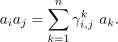
The segregation rates  are the structural constants of an
 -dimensional algebra. This is
provided in FriCAS by the constructor AlgebraGivenByStructuralConstants (abbreviation
ALGSC).
Consider two coupled autosomal loci with alleles  ,
 ,
 , and
 , building four different gametes
 and
 . The zygotes
 produce gametes
 and
 with classical
Mendelian segregation. Zygote
 undergoes transition to
 and vice versa with probability
 .
Define a list  of four four-by-four matrices giving the segregation rates. We use the value
 for
 .
segregationRates : List SquareMatrix(4,FRAC INT) := [matrix [ [1, 1/2, 1/2, 9/20], [1/2, 0, 1/20, 0], [1/2, 1/20, 0, 0], [9/20, 0, 0, 0] ], matrix [ [0, 1/2, 0, 1/20], [1/2, 1, 9/20, 1/2], [0, 9/20, 0, 0], [1/20, 1/2, 0, 0] ], matrix [ [0, 0, 1/2, 1/20], [0, 0, 9/20, 0], [1/2, 9/20, 1, 1/2], [1/20, 0, 1/2, 0] ], matrix [ [0, 0, 0, 9/20], [0, 0, 1/20, 1/2], [0, 1/20, 0, 1/2], [9/20, 1/2, 1/2, 1] ] ]
List(SquareMatrix(4, Fraction(Integer))) Choose the appropriate symbols for the basis of gametes,
gametes := [’AB,’Ab,’aB,’ab]
List(OrderedVariableList([AB, Ab, aB, ab])) Define the algebra.
A := ALGSC(FRAC INT, 4, gametes, segregationRates);
What are the probabilities for zygote  to produce the different gametes?
a := basis()$A; a.1*a.4
Elements in this algebra whose coefficients sum to one play a distinguished role. They represent a population with the distribution of gametes reflected by the coefficients with respect to the basis of gametes.
Random mating of different populations  and
 is described by their product
 .
This product is commutative only if the gametes are not sex-dependent, as in our example.
commutative?()$A
Boolean In general, it is not associative.
associative?()$A
Random mating within a population  is described by
 The next generation is

Use decimal numbers to compare the distributions more easily.
x : ALGSC(DECIMAL, 4, gametes, segregationRates) := convert [3/10, 1/5, 1/10, 2/5]
AlgebraGivenByStructuralConstants(DecimalExpansion, 4, [AB, Ab, aB, ab], [[[1, 0.5, 0.5, 0.45], [0.5, 0, 0.05, 0], [0.5, 0.05, 0, 0], [0.45, 0, 0, 0]], [[0, 0.5, 0, 0.05], [0.5, 1, 0.45, 0.5], [0, 0.45, 0, 0], [0.05, 0.5, 0, 0]], [[0, 0, 0.5, 0.05], [0, 0, 0.45, 0], [0.5, 0.45, 1, 0.5], [0.05, 0, 0.5, 0]], [[0, 0, 0, 0.45], [0, 0, 0.05, 0.5], [0, 0.05, 0, 0.5], [0.45, 0.5, 0.5, 1]]]) To compute directly the gametic distribution in the fifth generation, we use plenaryPower.
plenaryPower(x,5)
We now ask two questions: Does this distribution converge to an equilibrium state? What are the distributions that are stable?
This is an invariant of the algebra and it is used to answer the first question. The new indeterminates describe a symbolic distribution.
q := leftRankPolynomial()$GCNAALG(FRAC INT, 4, gametes, segregationRates) :: UP(Y, POLY FRAC INT)
UnivariatePolynomial(Y, Polynomial(Fraction(Integer))) Because the coefficient  has absolute value less than 1, all distributions
do converge, by a theorem of this theory.
factor(q :: POLY FRAC INT)
Factored(Polynomial(Fraction(Integer))) The second question is answered by searching for idempotents in the algebra.
cI := conditionsForIdempotents()$GCNAALG(FRAC INT, 4, gametes, segregationRates)
List(Polynomial(Fraction(Integer))) Solve these equations and look at the first solution.
gbs:= groebnerFactorize cI; gbs.1
List(Polynomial(Fraction(Integer)))
Further analysis using the package PolynomialIdeal shows that there is a two-dimensional variety of equilibrium states and all other solutions are contained in it.
Choose one equilibrium state by setting two indeterminates to concrete values.
sol := solve concat(gbs.1,[%x1-1/10,%x2-1/10])
List(List(Equation(Fraction(Polynomial(Integer)))))
e : A := represents reverse (map(rhs, sol.1) :: List FRAC INT)
e*e-e
This section shows some examples on selecting various (rectangular) submatrices of matrices. In the numerics literature, these operations are usually referred to as slicing. Apart from indexing matrices by two integers for retrieving single elements, it is possible to use lists of integers (List(Integer)), segments (Segment(Integer)) and list of segments (List(Segment(Integer))) to select slices like whole rows, columns or submatrices.
First, we build a simple test matrix to show the above-mentioned manipulations:
m := matrix([[11, 12, 13, 14], [21, 22,23, 24], [31, 32, 33, 34]])
Select the top right two by two submatrix by slicing using segments:
m(1..2, 3..4)
Having a nonzero step size in the segment is also supported:
m(1..2, 1..3 by 2)
Indexing by lists works as expected, returning all elements having index pairs from the outer product of both lists:
m([1,3], [2,4])
Selecting single elements by any index type other than Integer for both, the row and column index, will not give the respective element but a 1 times 1 matrix containing it:
m(1, 2)
m([1], [2])
m(1, [2])
m(1, 2..2)
m(1, [2..2])
It is possible to use lists of segments to select multiple submatrices which get stacked together forming the result returned:
m([1..2], [1, 3..4])
Use overlapping segments to repeat elements:
m([1..2], [3..4, 3..4])
It is even possible to mix any of the valid index constructs in the selection of rows and columns:
m(2, [1,4])
m([1,2,3], 2..3)
m([1,2], [1..3, 4])
Assignment to a submatrix using slicing syntax is supported, too:
m([1..2], [3..3]) := m([1,2], [2])
m
Note that assignment currently does not check for overlapping segments, and the last assignment wins. However, overlapping case should be considered undefined anyway.
Another caveat shows up when assigning single elements.
Selecting the entry by any index type other than two times an Integer requires assignment of a matrix type:
m([2], [2]) := matrix([[4]])
m
By using the functions rowSlice and colSlice it is possible to obtain for a given matrix two special slicing objects that when used will select all elements along a column or row respectively (rowSlice varies row index giving a column). The advantage of using these is that no information about the actual matrix size is necessary.
It is easily possible to select the second and fourth columns of a given matrix:
r := rowSlice(m)
m(r, 2)
m(r, 4)
Assignment of course works the same way. The following snippet shows simple row operations as used in Gaussian elimination:
c := colSlice(m)
m := m :: Matrix(Fraction(Integer))
m(2, c) := m(2, c) - m(2,1)/m(1,1) * m(1, c)
m(3, c) := m(3, c) - m(3,1)/m(1,1) * m(1, c)
m(3, c) := m(3, c) - m(3,2)/m(2,2) * m(2, c)
m
Selecting the whole matrix:
r := rowSlice(m)
c := colSlice(m)
m(r,c)
In this chapter we show examples of many of the most commonly used FriCAS domains and packages. The sections are organized by constructor names.
The AssociationList constructor provides a general structure for associative storage. This type provides association lists in which data objects can be saved according to keys of any type. For a given association list, specific types must be chosen for the keys and entries. You can think of the representation of an association list as a list of records with key and entry fields.
Association lists are a form of table and so most of the operations available for Table are also available for AssociationList. They can also be viewed as lists and can be manipulated accordingly.
This is a Record type with age and gender fields.
Data := Record(monthsOld : Integer, gender : String)
Type In this expression, al is declared to be an association list whose keys are strings and whose entries
are the above records.
al : AssociationList(String,Data)
The table operation is used to create an empty association list.
al := table()
AssociationList(String, Record(monthsOld: Integer, gender: String)) You can use assignment syntax to add things to the association list.
al."bob" := [407,"male"]$Data
Record(monthsOld: Integer, gender: String)
al."judith" := [366,"female"]$Data
Record(monthsOld: Integer, gender: String)
al."katie" := [24,"female"]$Data
Record(monthsOld: Integer, gender: String) Perhaps we should have included a species field.
al."smokie" := [200,"female"]$Data
Record(monthsOld: Integer, gender: String) Now look at what is in the association list. Note that the last-added (key, entry) pair is at the beginning of the list.
al
AssociationList(String, Record(monthsOld: Integer, gender: String)) You can reset the entry for an existing key.
al."katie" := [23,"female"]$Data
Record(monthsOld: Integer, gender: String) Use delete! to destructively remove an element of the association list. Use delete to return a copy of the association list with the element deleted. The second argument is the index of the element to delete.
delete!(al,1)
AssociationList(String, Record(monthsOld: Integer, gender: String))
For more information about tables, see ‘Table’ on page 1330. For more information about lists, see ‘List’ on page 1074. Issue the system command )show AssociationList to display the full list of operations defined by AssociationList.
BalancedBinaryTree(S) is the domain of balanced binary trees with elements of type S at the nodes. A
binary tree is either empty or else consists of a node having a value and two branches, each branch a binary
tree. A balanced binary tree is one that is balanced with respect to its leaves. One with  leaves is perfectly
“balanced”: the tree has minimum depth, and the left and right branch of every interior node is identical in
shape.
Balanced binary trees are useful in algebraic computation for so-called “divide-and-conquer” algorithms. Conceptually, the data for a problem is initially placed at the root of the tree. The original data is then split into two subproblems, one for each subtree. And so on. Eventually, the problem is solved at the leaves of the tree. A solution to the original problem is obtained by some mechanism that can reassemble the pieces. In fact, an implementation of the Chinese Remainder Algorithm using balanced binary trees was first proposed by David Y. Y. Yun at the IBM T. J. Watson Research Center in Yorktown Heights, New York, in 1978. It served as the prototype for polymorphic algorithms in FriCAS.
In what follows, rather than perform a series of computations with a single expression, the expression is
reduced modulo a number of integer primes, a computation is done with modular arithmetic for each prime,
and the Chinese Remainder Algorithm is used to obtain the answer to the original problem. We illustrate this
principle with the computation of  .
A list of moduli.
lm := [3,5,7,11]
List(PositiveInteger) The expression modTree(n, lm) creates a balanced binary tree with leaf values n mod m for each
modulus m in lm.
modTree(12,lm)
List(Integer) Operation modTree does this using operations on balanced binary trees. We trace its steps.
Create a balanced binary tree t of zeros with four leaves.
t := balancedBinaryTree(#lm, 0)
BalancedBinaryTree(NonNegativeInteger) The leaves of the tree are set to the individual moduli.
setleaves!(t,lm)
BalancedBinaryTree(NonNegativeInteger) Use mapUp! to do a bottom-up traversal of t, setting each interior node to the
product of the values at the nodes of its children.
mapUp!(t,_*)
PositiveInteger The value at the node of every subtree is the product of the moduli of the leaves of the subtree.
t
BalancedBinaryTree(NonNegativeInteger) Operation mapDown!(t,a,fn) replaces the value v at each node of t by
fn(a,v).
mapDown!(t,12,_rem)
BalancedBinaryTree(NonNegativeInteger) The operation leaves returns the leaves of the resulting tree. In this case, it
returns the list of 12 mod m for each modulus m.
leaves %
List(NonNegativeInteger) Compute the square of the images of 12 modulo each m.
squares := [x^2 rem m for x in % for m in lm]
List(NonNegativeInteger) Call the Chinese Remainder Algorithm to get the answer for  .
chineseRemainder(%,lm)
A basic operator is an object that can be symbolically applied to a list of arguments from a set, the result being a kernel over that set or an expression. In addition to this section, please see ‘Expression’ on page 847 and ‘Kernel’ on page 989 for additional information and examples.
You create an object of type BasicOperator by using the operator operation. This first form of this operation has one argument and it must be a symbol. The symbol should be quoted in case the name has been used as an identifier to which a value has been assigned.
A frequent application of BasicOperator is the creation of an operator to represent the unknown function
when solving a differential equation. Let y be the unknown function in terms of x.
y := operator ’y
BasicOperator This is how you enter the equation y’’ + y’ + y = 0.
deq := D(y x, x, 2) + D(y x, x) + y x = 0
Equation(Expression(Integer)) To solve the above equation, enter this.
solve(deq, y, x)
Union(Record(particular: Expression(Integer), basis: List(Expression(Integer))), ...) See Section 8.10 on page 581 for this kind of use of BasicOperator.
Use the single argument form of operator (as above) when you intend to use the operator to create functional expressions with an arbitrary number of arguments Nary means an arbitrary number of arguments can be used in the functional expressions.
nary? y
unary? y
Boolean Use the two-argument form when you want to restrict the number of arguments in the functional expressions created with the operator. This operator can only be used to create functional expressions with one argument.
opOne := operator(’opOne, 1)
nary? opOne
unary? opOne
Boolean Use arity to learn the number of arguments that can be used. It returns "false" if the operator is nary.
arity opOne
Union(NonNegativeInteger, ...) Use name to learn the name of an operator.
name opOne
Symbol Use is? to learn if an operator has a particular name.
is?(opOne, ’z2)
Boolean You can also use a string as the name to be tested against.
is?(opOne, "opOne")
You can attach named properties to an operator. These are rarely used at the top-level of the FriCAS interactive environment but are used with FriCAS library source code. By default, an operator has no properties.
properties y
AssociationList(Symbol, None) The interface for setting and getting properties is somewhat awkward because the property values are stored as values of type None. Attach a property by using setProperty.
setProperty(y, "use", "unknown function" :: None )
properties y
AssociationList(Symbol, None) We know the property value has type String.
property(y, "use") :: None pretend String
String Use deleteProperty! to destructively remove a property.
deleteProperty!(y, "use")
properties y
All rational numbers have repeating binary expansions. Operations to access the individual bits of a binary expansion can be obtained by converting the value to RadixExpansion(2). More examples of expansions are available in ‘DecimalExpansion’ on page 813, ‘HexadecimalExpansion’ on page 951, and ‘RadixExpansion’ on page 1208.
The expansion (of type BinaryExpansion) of a rational number is returned by the binary operation.
r := binary(22/7)
BinaryExpansion Arithmetic is exact.
r + binary(6/7)
BinaryExpansion The period of the expansion can be short or long …
[binary(1/i) for i in 102..106]
List(BinaryExpansion) or very long.
binary(1/1007)
BinaryExpansion These numbers are bona fide algebraic objects.
p := binary(1/4)*x^2 + binary(2/3)*x + binary(4/9)
q := D(p, x)
g := gcd(p, q)
BinarySearchTree(R) is the domain of binary trees with elements of type R, ordered across the nodes of the
tree. A non-empty binary search tree has a value of type R, and right and left binary search subtrees. If a
subtree is empty, it is displayed as a period (“.”).
Define a list of values to be placed across the tree. The resulting tree has 8 at the root; all other elements are
in the left subtree.
lv := [8,3,5,4,6,2,1,5,7]
List(PositiveInteger) A convenient way to create a binary search tree is to apply the operation binarySearchTree to a list of elements.
t := binarySearchTree lv
BinarySearchTree(PositiveInteger) Another approach is to first create an empty binary search tree of integers.
emptybst := empty()$BSTREE(INT)
BinarySearchTree(Integer) Insert the value 8. This establishes 8 as the root of the binary search
tree. Values inserted later that are less than 8 get stored in the left subtree, others in the right
subtree.
t1 := insert!(8,emptybst)
BinarySearchTree(Integer) Insert the value 3. This number becomes the root of the left subtree of t1. For
optimal retrieval, it is thus important to insert the middle elements first.
insert!(3,t1)
BinarySearchTree(Integer) We go back to the original tree t. The leaves of the binary search tree are those
which have empty left and right subtrees.
leaves t
List(PositiveInteger) The operation split(k,t) returns a record containing the two subtrees: one with all elements
“less” than k, another with elements “greater” than k.
split(3,t)
Record(less: BinarySearchTree(PositiveInteger), greater: BinarySearchTree(PositiveInteger)) Define insertRoot to insert new elements by creating a new node.
insertRoot: (INT,BSTREE INT) -> BSTREE INT
The new node puts the inserted value between its “less” tree and “greater” tree.
insertRoot(x, t) == a := split(x, t) node(a.less, x, a.greater)
Function buildFromRoot builds a binary search tree from a list of elements ls and the empty tree
emptybst.
buildFromRoot ls == reduce(insertRoot,ls,emptybst)
Apply this to the reverse of the list lv.
rt := buildFromRoot reverse lv
Compiling function buildFromRoot with type List(PositiveInteger) -> BinarySearchTree(Integer)
Compiling function insertRoot with type (Integer, BinarySearchTree(Integer)) -> BinarySearchTree(Integer)
BinarySearchTree(Integer) Have FriCAS check that these are equal.
(t = rt)@Boolean
The CardinalNumber domain can be used for values indicating the cardinality of sets, both finite and infinite.
The non-negative integers have a natural construction as cardinals
0 = #{ }, 1 = {0}, 2 = {0, 1}, ..., n = {i | 0 <= i < n}.
The fact that 0 acts as a zero for the multiplication of cardinals is equivalent to the axiom of
choice.
Cardinal numbers can be created by conversion from non-negative integers.
c0 := 0 :: CardinalNumber
c1 := 1 :: CardinalNumber
c2 := 2 :: CardinalNumber
c3 := 3 :: CardinalNumber
CardinalNumber They can also be obtained as the named cardinal Aleph(n).
A0 := Aleph 0
A1 := Aleph 1
CardinalNumber The finite? operation tests whether a value is a finite cardinal, that is, a non-negative integer.
finite? c2
finite? A0
Boolean Similarly, the countable? operation determines whether a value is a countable cardinal, that is,
finite or Aleph(0).
countable? c2
countable? A0
countable? A1
Boolean Arithmetic operations are defined on cardinal numbers as follows: If x = #X and y = #Y
then
x+y = #(X+Y) cardinality of the disjoint union x-y = #(X-Y) cardinality of the relative complement x*y = #(X*Y) cardinality of the Cartesian product x^y = #(X^Y) cardinality of the set of maps from Y to X
Here are some arithmetic examples.
[c2 + c2, c2 + A1]
[c0*c2, c1*c2, c2*c2, c0*A1, c1*A1, c2*A1, A0*A1]
[c2^c0, c2^c1, c2^c2, A1^c0, A1^c1, A1^c2]
List(CardinalNumber) Subtraction is a partial operation: it is not defined when subtracting a larger cardinal from a smaller one, nor when subtracting two equal infinite cardinals.
[c2-c1, c2-c2, c2-c3, A1-c2, A1-A0, A1-A1]
List(Union(CardinalNumber, "failed")) The generalized continuum hypothesis asserts that
2^Aleph i = Aleph(i+1)
and is independent of the axioms of set theory.1 The CardinalNumber domain provides an operation to assert whether the hypothesis is to be assumed.
generalizedContinuumHypothesisAssumed true
Boolean When the generalized continuum hypothesis is assumed, exponentiation to a transfinite power is allowed.
[c0^A0, c1^A0, c2^A0, A0^A0, A0^A1, A1^A0, A1^A1]
Three commonly encountered cardinal numbers are
 | countable infinity |
 | the continuum |
 |
In this domain, these values are obtained under the generalized continuum hypothesis in this way.
a := Aleph 0
c := 2^a
f := 2^c
CartesianTensor(i0,dim,R) provides Cartesian tensors with components belonging to a commutative ring
R. Tensors can be described as a generalization of vectors and matrices. This gives a concise tensor algebra for
multilinear objects supported by the CartesianTensor domain. You can form the inner or outer product of
any two tensors and you can add or subtract tensors with the same number of components. Additionally,
various forms of traces and transpositions are useful.
The CartesianTensor constructor allows you to specify the minimum index for subscripting. In what follows we discuss in detail how to manipulate tensors.
Here we construct the domain of Cartesian tensors of dimension 2 over the integers, with indices starting at 1.
CT := CARTEN(i0 := 1, 2, Integer)
Scalars can be converted to tensors of rank zero.
t0: CT := 8
CartesianTensor(1, 2, Integer)
rank t0
NonNegativeInteger Vectors (mathematical direct products, rather than one dimensional array structures) can be converted to tensors of rank one.
v: DirectProduct(2, Integer) := directProduct [3,4]
Tv: CT := v
CartesianTensor(1, 2, Integer) Matrices can be converted to tensors of rank two.
m: SquareMatrix(2, Integer) := matrix [[1,2],[4,5]]
Tm: CT := m
CartesianTensor(1, 2, Integer)
n: SquareMatrix(2, Integer) := matrix [[2,3],[0,1]]
Tn: CT := n
CartesianTensor(1, 2, Integer) In general, a tensor of rank k can be formed by making a list of rank k-1 tensors
or, alternatively, a k-deep nested list of lists.
t1: CT := [2, 3]
CartesianTensor(1, 2, Integer)
rank t1
t2: CT := [t1, t1]
CartesianTensor(1, 2, Integer)
t3: CT := [t2, t2]
CartesianTensor(1, 2, Integer)
tt: CT := [t3, t3]; tt := [tt, tt]
CartesianTensor(1, 2, Integer)
rank tt
Given two tensors of rank k1 and k2, the outer product forms a new tensor of rank k1+k2. Here

Tmn := product(Tm, Tn)
CartesianTensor(1, 2, Integer)
The inner product (contract) forms a tensor of rank k1+k2-2. This product generalizes the vector dot product
and matrix-vector product by summing component products along two indices. Here we sum along the
second index of  and the first index of
 . Here

Tmv := contract(Tm,2,Tv,1)
CartesianTensor(1, 2, Integer)
The multiplication operator * is scalar multiplication or an inner product depending on the ranks of the
arguments. If either argument is rank zero it is treated as scalar multiplication. Otherwise, a*b is the inner
product summing the last index of a with the first index of b.
Tm*Tv
CartesianTensor(1, 2, Integer) This definition is consistent with the inner product on matrices and vectors.
Tmv = m * v
Equation(CartesianTensor(1, 2, Integer))
For tensors of low rank (that is, four or less), components can be selected by applying the tensor to its indices.
t0()
t1(1+1)
t2(2,1)
t3(2,1,2)
Tmn(2,1,2,1)
NonNegativeInteger A general indexing mechanism is provided for a list of indices.
t0[]
t1[2]
t2[2,1]
PositiveInteger The general mechanism works for tensors of arbitrary rank, but is somewhat less efficient since the intermediate index list must be created.
t3[2,1,2]
Tmn[2,1,2,1]
A “contraction” between two tensors is an inner product, as we have seen above. You can also contract a
pair of indices of a single tensor. This corresponds to a “trace” in linear algebra. The expression
contract(t,k1,k2) forms a new tensor by summing the diagonal given by indices in position k1 and k2.
This is the tensor given by 
cTmn := contract(Tmn,1,2)
CartesianTensor(1, 2, Integer) Since Tmn is the outer product of matrix m and matrix n, the above is equivalent
to this.
trace(m) * n
SquareMatrix(2, Integer) In this and the next few examples, we show all possible contractions of Tmn and their
matrix algebra equivalents.
contract(Tmn,1,2) = trace(m) * n
Equation(CartesianTensor(1, 2, Integer))
contract(Tmn,1,3) = transpose(m) * n
Equation(CartesianTensor(1, 2, Integer))
contract(Tmn,1,4) = transpose(m) * transpose(n)
Equation(CartesianTensor(1, 2, Integer))
contract(Tmn,2,3) = m * n
Equation(CartesianTensor(1, 2, Integer))
contract(Tmn,2,4) = m * transpose(n)
Equation(CartesianTensor(1, 2, Integer))
contract(Tmn,3,4) = trace(n) * m
Equation(CartesianTensor(1, 2, Integer))
You can exchange any desired pair of indices using the transpose operation.
Here the indices in positions one and three are exchanged, that is, 
tTmn := transpose(Tmn,1,3)
CartesianTensor(1, 2, Integer) If no indices are specified, the first and last index are exchanged.
transpose Tmn
CartesianTensor(1, 2, Integer) This is consistent with the matrix transpose.
transpose Tm = transpose m
Equation(CartesianTensor(1, 2, Integer))
If a more complicated reordering of the indices is required, then the reindex operation can be used. This
operation allows the indices to be arbitrarily permuted. This defines 
rTmn := reindex(Tmn, [1,4,2,3])
CartesianTensor(1, 2, Integer)
Tensors of equal rank can be added or subtracted so arithmetic expressions can be used to produce new tensors.
tt := transpose(Tm)*Tn - Tn*transpose(Tm)
CartesianTensor(1, 2, Integer)
Tv*(tt+Tn)
CartesianTensor(1, 2, Integer)
reindex(product(Tn,Tn),[4,3,2,1])+3*Tn*product(Tm,Tm)
CartesianTensor(1, 2, Integer)
Two specific tensors have properties which depend only on the dimension.
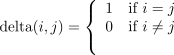
delta: CT := kroneckerDelta()
CartesianTensor(1, 2, Integer) This can be used to reindex via contraction.
contract(Tmn, 2, delta, 1) = reindex(Tmn, [1,3,4,2])
Equation(CartesianTensor(1, 2, Integer))
The Levi Civita symbol determines the sign of a permutation of indices.
epsilon:CT := leviCivitaSymbol()
CartesianTensor(1, 2, Integer) Here we have:
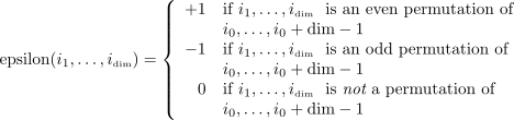
This property can be used to form determinants.
contract(epsilon*Tm*epsilon, 1,2) = 2 * determinant m
Equation(CartesianTensor(1, 2, Integer))
GradedModule(R,E) denotes “E-graded R-module”, that is, a collection of R-modules indexed by an abelian
monoid E. An element g of G[s] for some specific s in E is said to be an element of G with degree s. Sums are
defined in each module G[s] so two elements of G can be added if they have the same degree.
Morphisms can be defined and composed by degree to give the mathematical category of graded
modules.
GradedAlgebra(R,E) denotes “E-graded R-algebra.” A graded algebra is a graded module together with a
degree preserving R-bilinear map, called the product.
degree(product(a,b))= degree(a) + degree(b) product(r*a,b) = product(a,r*b) = r*product(a,b) product(a1+a2,b) = product(a1,b) + product(a2,b) product(a,b1+b2) = product(a,b1) + product(a,b2) product(a,product(b,c)) = product(product(a,b),c)
The domain CartesianTensor(i0, dim, R) belongs to the category GradedAlgebra(R, NonNegativeInteger). The non-negative integer degree is the tensor rank and the graded algebra product is the tensor outer product. The graded module addition captures the notion that only tensors of equal rank can be added.
If V is a vector space of dimension dim over R, then the tensor module T[k](V) is defined as
T[0](V) = R T[k](V) = T[k-1](V) * V
where * denotes the R-module tensor product. CartesianTensor(i0,dim,R) is the graded algebra in which
the degree k module is T[k](V).
It should be noted here that often tensors are used in the context of tensor-valued manifold maps. This leads to the notion of covariant and contravariant bases with tensor component functions transforming in specific ways under a change of coordinates on the manifold. This is no more directly supported by the CartesianTensor domain than it is by the Vector domain. However, it is possible to have the components implicitly represent component maps by choosing a polynomial or expression type for the components. In this case, it is up to the user to satisfy any constraints which arise on the basis of this interpretation.
The members of the domain Character are values representing letters, numerals and other text elements. For more information on related topics, see ‘CharacterClass’ on page 751 and ‘String’ on page 1304.
Characters can be obtained using String notation.
chars := [char "a", char "A", char "X", char "8", char "+"]
List(Character) Certain characters are available by name. This is the blank character.
space()
Character This is the quote that is used in strings.
quote()
Character This is the underscore character which is used to allow quotes and other special characters within strings.
underscore()
Character Characters are represented as integers in a machine-dependent way. The integer value can be
obtained using the ord operation. It is always true that char(ord c)= c and ord(char i)= i, provided that i is
in the range 0..size()$Character-1.
[ord c for c in chars]
The lowerCase operation converts an upper case letter to the corresponding lower case letter. If the argument is not an upper case letter, then it is returned unchanged.
[upperCase c for c in chars]
List(Character) Likewise, the upperCase operation converts lower case letters to upper case.
[lowerCase c for c in chars]
A number of tests are available to determine whether characters belong to certain families.
[alphabetic? c for c in chars]
[upperCase? c for c in chars]
[lowerCase? c for c in chars]
[digit? c for c in chars]
[hexDigit? c for c in chars]
[alphanumeric? c for c in chars]
The CharacterClass domain allows classes of characters to be defined and manipulated efficiently.
Character classes can be created by giving either a string or a list of characters.
cl1 := charClass [char "a", char "e", char "i", char "o", char "u", char "y"]
cl2 := charClass "bcdfghjklmnpqrstvwxyz"
CharacterClass A number of character classes are predefined for convenience.
digit()
hexDigit()
upperCase()
lowerCase()
alphabetic()
alphanumeric()
CharacterClass You can quickly test whether a character belongs to a class.
member?(char "a", cl1)
member?(char "a", cl2)
Boolean Classes have the usual set operations because the CharacterClass domain belongs to the category FiniteSetAggregate(Character).
intersect(cl1, cl2)
union(cl1,cl2)
difference(cl1,cl2)
intersect(complement(cl1),cl2)
CharacterClass You can modify character classes by adding or removing characters.
insert!(char "a", cl2)
remove!(char "b", cl2)
For more information on related topics, see ‘Character’ on page 745 and ‘String’ on page 1304. Issue the system command )show CharacterClass to display the full list of operations defined by CharacterClass.
CliffordAlgebra(n,K,Q) defines a vector space of dimension  over the field
 with a given bilinear
form represented by a square matrix
Q. If  is a basis for
 then
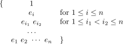
is a basis for the Clifford algebra. The algebra is defined by the relation

for all  being linear combinations of
 . Examples of Clifford Algebras are gaussians (complex numbers),
quaternions, exterior algebras and spin algebras.
This is the field over which we will work, rational functions with integer coefficients.
K := Fraction Polynomial Integer
Type We use this matrix for the quadratic form.
m := matrix [[-1]]
Matrix(Integer) We get complex arithmetic by using this domain.
C := CliffordAlgebra(1, K, m)
Type Here is i, the usual square root of -1.
i: C := e(1)
CliffordAlgebra(1, Fraction(Polynomial(Integer)), [[-1]]) Here are some examples of the arithmetic.
x := a + b * i
CliffordAlgebra(1, Fraction(Polynomial(Integer)), [[-1]])
y := c + d * i
CliffordAlgebra(1, Fraction(Polynomial(Integer)), [[-1]]) See ‘Complex’ on page 774 for examples of FriCAS’s constructor implementing complex numbers.
x * y
CliffordAlgebra(1, Fraction(Polynomial(Integer)), [[-1]])
This is the field over which we will work, rational functions with integer coefficients.
K := Fraction Polynomial Integer
Type We use this matrix for the quadratic form.
m := matrix [[-1,0],[0,-1]]
Matrix(Integer) The resulting domain is the quaternions.
H := CliffordAlgebra(2, K, m)
Type We use Hamilton’s notation for i,j,k.
i: H := e(1)
CliffordAlgebra(2, Fraction(Polynomial(Integer)), [[-1, 0], [0, -1]])
j: H := e(2)
CliffordAlgebra(2, Fraction(Polynomial(Integer)), [[-1, 0], [0, -1]])
k: H := i * j
CliffordAlgebra(2, Fraction(Polynomial(Integer)), [[-1, 0], [0, -1]])
x := a + b * i + c * j + d * k
CliffordAlgebra(2, Fraction(Polynomial(Integer)), [[-1, 0], [0, -1]])
y := e + f * i + g * j + h * k
CliffordAlgebra(2, Fraction(Polynomial(Integer)), [[-1, 0], [0, -1]])
x + y
CliffordAlgebra(2, Fraction(Polynomial(Integer)), [[-1, 0], [0, -1]])
x * y
CliffordAlgebra(2, Fraction(Polynomial(Integer)), [[-1, 0], [0, -1]]) See ‘Quaternion’ on page 1203 for examples of FriCAS’s constructor implementing quaternions.
y * x
CliffordAlgebra(2, Fraction(Polynomial(Integer)), [[-1, 0], [0, -1]])
This is the field over which we will work, rational functions with integer coefficients.
K := Fraction Polynomial Integer
Type If we choose the three by three zero quadratic form, we obtain the exterior algebra on
e(1),e(2),e(3).
Ext := CliffordAlgebra(3, K, 0)
Type This is a three dimensional vector algebra. We define i, j, k as the unit vectors.
i: Ext := e(1)
CliffordAlgebra(3, Fraction(Polynomial(Integer)), [[0, 0, 0], [0, 0, 0], [0, 0, 0]])
j: Ext := e(2)
CliffordAlgebra(3, Fraction(Polynomial(Integer)), [[0, 0, 0], [0, 0, 0], [0, 0, 0]])
k: Ext := e(3)
CliffordAlgebra(3, Fraction(Polynomial(Integer)), [[0, 0, 0], [0, 0, 0], [0, 0, 0]]) Now it is possible to do arithmetic.
x := x1*i + x2*j + x3*k
CliffordAlgebra(3, Fraction(Polynomial(Integer)), [[0, 0, 0], [0, 0, 0], [0, 0, 0]])
y := y1*i + y2*j + y3*k
CliffordAlgebra(3, Fraction(Polynomial(Integer)), [[0, 0, 0], [0, 0, 0], [0, 0, 0]])
x + y
CliffordAlgebra(3, Fraction(Polynomial(Integer)), [[0, 0, 0], [0, 0, 0], [0, 0, 0]])
x * y + y * x
CliffordAlgebra(3, Fraction(Polynomial(Integer)), [[0, 0, 0], [0, 0, 0], [0, 0, 0]]) On an n space, a grade p form has a dual n-p form. In particular, in three space
the dual of a grade two element identifies e1*e2.
 e3, e2*e3
 e1, e3*e1
 e2
dual2 a == coefficient(a,[2,3]) * i + coefficient(a,[3,1]) * j + coefficient(a,[1,2]) * k
The vector cross product is then given by this.
dual2(x*y)
Compiling function dual2 with type CliffordAlgebra(3,Fraction(Polynomial( Integer)),[[0,0,0],[0,0,0],[0,0,0]]) -> CliffordAlgebra(3,Fraction( Polynomial(Integer)),[[0,0,0],[0,0,0],[0,0,0]])
CliffordAlgebra(3, Fraction(Polynomial(Integer)), [[0, 0, 0], [0, 0, 0], [0, 0, 0]])
In this section we will work over the field of rational numbers.
K := Fraction Integer
Type We define the quadratic form to be the Minkowski space-time metric.
g := matrix [[1,0,0,0], [0,-1,0,0], [0,0,-1,0], [0,0,0,-1]]
Matrix(Integer) We obtain the Dirac spin algebra used in Relativistic Quantum Field Theory.
D := CliffordAlgebra(4, K, g)
Type The usual notation for the basis is  with a superscript. For FriCAS input we will use
gam(i):
gam := [e(i)$D for i in 1..4]
List(CliffordAlgebra(4, Fraction(Integer), [[1, 0, 0, 0], [0, -1, 0, 0], [0, 0, -1, 0], [0, 0, 0, -1]])) There are various contraction identities of the form
g(l,t)*gam(l)*gam(m)*gam(n)*gam(r)*gam(s)*gam(t) = 2*(gam(s)gam(m)gam(n)gam(r) + gam(r)*gam(n)*gam(m)*gam(s))
where a sum over l and t is implied. Verify this identity for particular values of m,n,r,s.
m := 1; n:= 2; r := 3; s := 4;
lhs := reduce(+, [reduce(+, [ g(l,t)*gam(l)*gam(m)*gam(n)*gam(r)*gam(s)*gam(t) for l in 1..4]) for t in 1..4])
CliffordAlgebra(4, Fraction(Integer), [[1, 0, 0, 0], [0, -1, 0, 0], [0, 0, -1, 0], [0, 0, 0, -1]])
rhs := 2*(gam s * gam m*gam n*gam r + gam r*gam n*gam m*gam s)
CliffordAlgebra(4, Fraction(Integer), [[1, 0, 0, 0], [0, -1, 0, 0], [0, 0, -1, 0], [0, 0, 0, -1]])
The Complex constructor implements complex objects over a commutative ring R. Typically, the ring R is
Integer, Fraction Integer, Float or DoubleFloat. R can also be a symbolic type, like Polynomial
Integer. For more information about the numerical and graphical aspects of complex numbers, see Section
8.1 on page 479.
Complex objects are created by the complex operation.
a := complex(4/3,5/2)
b := complex(4/3,-5/2)
Complex(Fraction(Integer)) The standard arithmetic operations are available.
a + b
a - b
a * b
Complex(Fraction(Integer)) If R is a field, you can also divide the complex objects.
a / b
Complex(Fraction(Integer)) Use a conversion (Section 2.7 on page 167) to view the last object as a fraction of complex integers.
% :: Fraction Complex Integer
Fraction(Complex(Integer)) The predefined macro %i is defined to be complex(0,1).
3.4 + 6.7 * %i
Complex(Float) You can also compute the conjugate and norm of a complex number.
conjugate a
norm a
Fraction(Integer) The real and imag operations are provided to extract the real and imaginary parts, respectively.
real a
imag a
The domain Complex Integer is also called the Gaussian integers. If R is the integers (or, more generally, a
EuclideanDomain), you can compute greatest common divisors.
gcd(13 - 13*%i,31 + 27*%i)
Complex(Integer) You can also compute least common multiples.
lcm(13 - 13*%i,31 + 27*%i)
Complex(Integer) You can factor Gaussian integers.
factor(13 - 13*%i)
factor complex(2,0)
Continued fractions have been a fascinating and useful tool in mathematics for well over three hundred years. FriCAS implements continued fractions for fractions of any Euclidean domain. In practice, this usually means rational numbers. In this section we demonstrate some of the operations available for manipulating both finite and infinite continued fractions. It may be helpful if you review ‘Stream’ on page 1300 to remind yourself of some of the operations with streams.
The ContinuedFraction domain is a field and therefore you can add, subtract, multiply and divide the fractions. The continuedFraction operation converts its fractional argument to a continued fraction.
c := continuedFraction(314159/100000)
ContinuedFraction(Integer) This display is a compact form of the bulkier
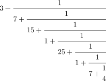
You can write any rational number in a similar form. The fraction will be finite and you can always take the
“numerators” to be 1. That is, any rational number can be written as a simple, finite continued fraction of the
form
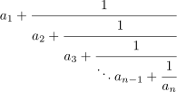
The  are called partial quotients and the operation partialQuotients creates a stream of them.
partialQuotients c
Stream(Integer) By considering more and more of the fraction, you get the convergents. For example, the
first convergent is  , the second is
 and so on.
convergents c
Stream(Fraction(Integer)) Since this is a finite continued fraction, the last convergent is the original rational number, in reduced form. The result of approximants is always an infinite stream, though it may just repeat the “last” value.
approximants c
Stream(Fraction(Integer)) Inverting c only changes the partial quotients of its fraction by inserting a 0 at the
beginning of the list.
pq := partialQuotients(1/c)
Stream(Integer) Do this to recover the original continued fraction from this list of partial quotients. The three-argument form of the continuedFraction operation takes an element which is the whole part of the fraction, a stream of elements which are the numerators of the fraction, and a stream of elements which are the denominators of the fraction.
continuedFraction(first pq,repeating [1],rest pq)
ContinuedFraction(Integer) The streams need not be finite for continuedFraction. Can you guess which irrational number has the following continued fraction? See the end of this section for the answer.
z:=continuedFraction(3,repeating [1],repeating [3,6])
In 1737 Euler discovered the infinite continued fraction expansion
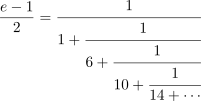
We use this expansion to compute rational and floating point approximations of
e.2
By looking at the above expansion, we see that the whole part is 0 and the numerators are all equal to 1. This
constructs the stream of denominators.
dens : Stream Integer := cons(1, stream((x +-> x + 4), 6))
Stream(Integer) Therefore this is the continued fraction expansion for  .
cf := continuedFraction(0,repeating [1],dens)
ContinuedFraction(Integer) These are the rational number convergents.
ccf := convergents cf
Stream(Fraction(Integer)) You can get rational convergents for e by multiplying by 2 and adding 1.
eConvergents := [2*e + 1 for e in ccf]
Stream(Fraction(Integer)) You can also compute the floating point approximations to these convergents.
eConvergents :: Stream Float
Stream(Float) Compare this to the value of e computed by the exp operation in Float.
exp 1.0
In about 1658, Lord Brouncker established the following expansion for  .
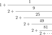
Let’s use this expansion to compute rational and floating point approximations for  .
cf := continuedFraction(1,[(2*i+1)^2 for i in 0..],repeating [2])
ccf := convergents cf
piConvergents := [4/p for p in ccf]
Stream(Fraction(Integer)) As you can see, the values are converging to  = 3.14159265358979323846..., but not very
quickly.
piConvergents :: Stream Float
You need not restrict yourself to continued fractions of integers. Here is an expansion for a quotient of Gaussian integers.
continuedFraction((- 122 + 597*%i)/(4 - 4*%i))
ContinuedFraction(Complex(Integer)) This is an expansion for a quotient of polynomials in one variable with rational number coefficients.
r : Fraction UnivariatePolynomial(x,Fraction Integer)
r := ((x - 1) * (x - 2)) / ((x-3) * (x-4))
Fraction(UnivariatePolynomial(x, Fraction(Integer)))
continuedFraction r
ContinuedFraction(UnivariatePolynomial(x, Fraction(Integer)))
To conclude this section, we give you evidence that
z
ContinuedFraction(Integer) is the expansion of  .
[i*i for i in convergents(z) :: Stream Float]
continuedFraction sqrt 11.0
This section is based upon the paper J. H. Redfield, “The Theory of Group-Reduced Distributions”, American J. Math.,49 (1927) 433-455, and is an application of group theory to enumeration problems. It is a development of the work by P. A. MacMahon on the application of symmetric functions and Hammond operators to combinatorial theory.
The theory is based upon the power sum symmetric functions  which are the sum of the
 powers of the
variables. The cycle index of a permutation is an expression that specifies the sizes of the cycles of a
permutation, and may be represented as a partition. A partition of a non-negative integer
n is a collection of
positive integers called its parts whose sum is n. For example, the partition  will be used to
represent
 and will indicate that the permutation has two cycles of length 3, one of length 2 and two of
length 1. The cycle index of a permutation group is the sum of the cycle indices of its permutations divided by
the number of permutations. The cycle indices of certain groups are provided. We first expose something
from the library.
)expose EVALCYC
EvaluateCycleIndicators is now explicitly exposed in frame initial
The operation complete returns the cycle index of the symmetric group of order n for argument n.
Alternatively, it is the  complete homogeneous symmetric function expressed in terms of power sum
symmetric functions.
complete 1
SymmetricPolynomial(Fraction(Integer))
complete 2
SymmetricPolynomial(Fraction(Integer))
complete 3
SymmetricPolynomial(Fraction(Integer))
complete 7
SymmetricPolynomial(Fraction(Integer)) The operation elementary computes the  elementary symmetric function
for argument
n.
elementary 7
SymmetricPolynomial(Fraction(Integer)) The operation alternating returns the cycle index of the alternating group having an even number of even parts in each cycle partition.
alternating 7
SymmetricPolynomial(Fraction(Integer)) The operation cyclic returns the cycle index of the cyclic group.
cyclic 7
SymmetricPolynomial(Fraction(Integer)) The operation dihedral is the cycle index of the dihedral group.
dihedral 7
SymmetricPolynomial(Fraction(Integer)) The operation graphs for argument n returns the cycle index of the group of
permutations on the edges of the complete graph with n nodes induced by applying the symmetric group to
the nodes.
graphs 5
SymmetricPolynomial(Fraction(Integer))
The cycle index of a direct product of two groups is the product of the cycle indices of the groups. Redfield provided two operations on two cycle indices which will be called “cup” and “cap” here. The cup of two cycle indices is a kind of scalar product that combines monomials for permutations with the same cycles. The cap operation provides the sum of the coefficients of the result of the cup operation which will be an integer that enumerates what Redfield called group-reduced distributions.
We can, for example, represent complete 2 * complete 2 as the set of objects a a b b and
complete 2 * complete 1 * complete 1 as c c d e.
This integer is the number of different sets of four pairs.
cap(complete 2^2, complete 2*complete 1^2)
Fraction(Integer) For example,
a a b b a a b b a a b b a a b b c c d e c d c e c e c d d e c c
This integer is the number of different sets of four pairs no two pairs being equal.
cap(elementary 2^2, complete 2*complete 1^2)
Fraction(Integer) For example,
a a b b a a b b c d c e c e c d
In this case the configurations enumerated are easily constructed, however the theory merely enumerates them
providing little help in actually constructing them. Here are the number of 6-pairs, first from a a a b b c,
second from d d e e f g.
cap(complete 3*complete 2*complete 1,complete 2^2*complete 1^2)
Fraction(Integer) Here it is again, but with no equal pairs.
cap(elementary 3*elementary 2*elementary 1,complete 2^2*complete 1^2)
cap(complete 3*complete 2*complete 1,elementary 2^2*elementary 1^2)
Fraction(Integer) The number of 6-triples, first from a a a b b c, second from d d e e f g, third from
h h i i j j.
eval(cup(complete 3*complete 2*complete 1, cup(complete 2^2*complete 1^2,complete 2^3)))
Fraction(Integer) The cycle index of vertices of a square is dihedral 4.
square:=dihedral 4
SymmetricPolynomial(Fraction(Integer)) The number of different squares with 2 red vertices and 2 blue vertices.
cap(complete 2^2,square)
Fraction(Integer) The number of necklaces with 3 red beads, 2 blue beads and 2 green beads.
cap(complete 3*complete 2^2,dihedral 7)
Fraction(Integer) The number of graphs with 5 nodes and 7 edges.
cap(graphs 5,complete 7*complete 3)
Fraction(Integer) The cycle index of rotations of vertices of a cube.
s(x) == powerSum(x)
cube:=(1/24)*(s 1^8+9*s 2^4 + 8*s 3^2*s 1^2+6*s 4^2)
Compiling function s with type PositiveInteger -> SymmetricPolynomial(Fraction( Integer))
SymmetricPolynomial(Fraction(Integer)) The number of cubes with 4 red vertices and 4 blue vertices.
cap(complete 4^2,cube)
Fraction(Integer) The number of labeled graphs with degree sequence 2 2 2 1 1 with no loops or multiple
edges.
cap(complete 2^3*complete 1^2,wreath(elementary 4,elementary 2))
Fraction(Integer) Again, but with loops allowed but not multiple edges.
cap(complete 2^3*complete 1^2,wreath(elementary 4,complete 2))
Fraction(Integer) Again, but with multiple edges allowed, but not loops
cap(complete 2^3*complete 1^2,wreath(complete 4,elementary 2))
Fraction(Integer) Again, but with both multiple edges and loops allowed
cap(complete 2^3*complete 1^2,wreath(complete 4,complete 2))
Having constructed a cycle index for a configuration we are at liberty to evaluate the  components any way
we please. For example we can produce enumerating generating functions. This is done by providing a
function
f on an integer i to the value required of  , and then evaluating
eval(f, cycleindex).
x: ULS(FRAC INT,’x,0) := ’x
UnivariateLaurentSeries(Fraction(Integer), x, 0)
ZeroOrOne: INT -> ULS(FRAC INT, ’x, 0)
Integers: INT -> ULS(FRAC INT, ’x, 0)
For the integers 0 and 1, or two colors.
ZeroOrOne n == 1+x^n
ZeroOrOne 5
Compiling function ZeroOrOne with type Integer -> UnivariateLaurentSeries( Fraction(Integer),x,0)
UnivariateLaurentSeries(Fraction(Integer), x, 0) For the integers 0, 1, 2, ... we have this.
Integers n == 1/(1-x^n)
Integers 5
Compiling function Integers with type Integer -> UnivariateLaurentSeries( Fraction(Integer),x,0)
UnivariateLaurentSeries(Fraction(Integer), x, 0)
The coefficient of  is the number of graphs with 5 nodes and
n edges.
eval(ZeroOrOne, graphs 5)
UnivariateLaurentSeries(Fraction(Integer), x, 0) The coefficient of  is the number of necklaces with
n red beads and
n-8 green beads.
eval(ZeroOrOne,dihedral 8)
UnivariateLaurentSeries(Fraction(Integer), x, 0) The coefficient of  is the number of partitions of
n into 4 or fewer
parts.
eval(Integers,complete 4)
UnivariateLaurentSeries(Fraction(Integer), x, 0) The coefficient of  is the number of partitions of
n into 4 boxes
containing ordered distinct parts.
eval(Integers,elementary 4)
UnivariateLaurentSeries(Fraction(Integer), x, 0) The coefficient of  is the number of different cubes with
n red vertices
and 8-n green ones.
eval(ZeroOrOne,cube)
UnivariateLaurentSeries(Fraction(Integer), x, 0) The coefficient of  is the number of different cubes with integers on
the vertices whose sum is
n.
eval(Integers,cube)
UnivariateLaurentSeries(Fraction(Integer), x, 0) The coefficient of  is the number of graphs with 5 nodes and with
integers on the edges whose sum is
n. In other words, the enumeration is of multigraphs with 5 nodes and n
edges.
eval(Integers,graphs 5)
UnivariateLaurentSeries(Fraction(Integer), x, 0) Graphs with 15 nodes enumerated with respect to number of edges.
eval(ZeroOrOne ,graphs 15)
UnivariateLaurentSeries(Fraction(Integer), x, 0) Necklaces with 7 green beads, 8 white beads, 5 yellow beads and 10 red beads.
cap(dihedral 30,complete 7*complete 8*complete 5*complete 10)
Fraction(Integer) The operation SFunction is the S-function or Schur function of a partition
written as a descending list of integers expressed in terms of power sum symmetric functions. In
this case the argument partition represents a tableau shape. For example 3,2,2,1 represents a
tableau with three boxes in the first row, two boxes in the second and third rows, and one box in
the fourth row. SFunction [3,2,2,1] counts the number of different tableaux of shape 3, 2, 2, 1
filled with objects with an ascending order in the columns and a non-descending order in the
rows.
sf3221:= SFunction [3,2,2,1]
SymmetricPolynomial(Fraction(Integer)) This is the number filled with a a b b c c d d.
cap(sf3221,complete 2^4)
Fraction(Integer) The configurations enumerated above are:
a a b a a c a a d b c b b b b c d c d c c d d d
This is the number of tableaux filled with 1..8.
cap(sf3221, powerSum 1^8)
Fraction(Integer) The coefficient of  is the number of column strict reverse plane partitions of
n of shape
3 2 2 1.
eval(Integers, sf3221)
UnivariateLaurentSeries(Fraction(Integer), x, 0) The smallest is
0 0 0 1 1 2 2 3
All rationals have repeating decimal expansions. Operations to access the individual digits of a decimal expansion can be obtained by converting the value to RadixExpansion(10). More examples of expansions are available in ‘BinaryExpansion’ on page 703, ‘HexadecimalExpansion’ on page 951, and ‘RadixExpansion’ on page 1208. Issue the system command )show DecimalExpansion to display the full list of operations defined by DecimalExpansion.
The operation decimal is used to create this expansion of type DecimalExpansion.
r := decimal(22/7)
DecimalExpansion Arithmetic is exact.
r + decimal(6/7)
DecimalExpansion The period of the expansion can be short or long …
[decimal(1/i) for i in 350..354]
List(DecimalExpansion) or very long.
decimal(1/2049)
DecimalExpansion These numbers are bona fide algebraic objects.
p := decimal(1/4)*x^2 + decimal(2/3)*x + decimal(4/9)
q := differentiate(p, x)
g := gcd(p, q)
The domain constructor DeRhamComplex creates the class of differential forms of arbitrary degree over a
coefficient ring. The De Rham complex constructor takes two arguments: a ring, coefRing, and a list of
coordinate variables.
This is the ring of coefficients.
coefRing := Integer
Type These are the coordinate variables.
lv : List Symbol := [x,y,z]
List(Symbol) This is the De Rham complex of Euclidean three-space using coordinates x, y and
z.
der := DERHAM(coefRing,lv)
This complex allows us to describe differential forms having expressions of integers as coefficients. These
coefficients can involve any number of variables, for example, f(x,t,r,y,u,z). As we’ve chosen to work with
ordinary Euclidean three-space, expressions involving these forms are treated as functions of x, y and z with
the additional arguments t, r and u regarded as symbolic constants. Here are some examples of
coefficients.
R := Expression coefRing
f : R := x^2*y*z-5*x^3*y^2*z^5
g : R := z^2*y*cos(z)-7*sin(x^3*y^2)*z^2
h : R :=x*y*z-2*x^3*y*z^2
Expression(Integer) We now define the multiplicative basis elements for the exterior algebra over
R.
dx : der := generator(1)
DeRhamComplex(Integer, [x, y, z])
dy : der := generator(2)
DeRhamComplex(Integer, [x, y, z])
dz : der := generator(3)
DeRhamComplex(Integer, [x, y, z]) This is an alternative way to give the above assignments.
[dx,dy,dz] := [generator(i)$der for i in 1..3]
List(DeRhamComplex(Integer, [x, y, z])) Now we define some one-forms.
alpha : der := f*dx + g*dy + h*dz
DeRhamComplex(Integer, [x, y, z])
beta : der := cos(tan(x*y*z)+x*y*z)*dx + x*dy
DeRhamComplex(Integer, [x, y, z]) A well-known theorem states that the composition of exteriorDifferential with
itself is the zero map for continuous forms. Let’s verify this theorem for alpha.
exteriorDifferential alpha;
DeRhamComplex(Integer, [x, y, z]) We suppressed the lengthy output of the last expression, but nevertheless, the composition is zero.
exteriorDifferential %
DeRhamComplex(Integer, [x, y, z])
Now we check that exteriorDifferential is a “graded derivation” D, that is, D satisfies:

gamma := alpha * beta
DeRhamComplex(Integer, [x, y, z]) We try this for the one-forms alpha and beta.
exteriorDifferential(gamma) - (exteriorDifferential(alpha)*beta - alpha * exteriorDifferential(beta))
DeRhamComplex(Integer, [x, y, z]) Now we define some “basic operators” (see ‘Operator’ on page 1151).
a : BOP := operator(’a)
b : BOP := operator(’b)
c : BOP := operator(’c)
BasicOperator We also define some indeterminate one- and two-forms using these operators.
sigma := a(x,y,z) * dx + b(x,y,z) * dy + c(x,y,z) * dz
DeRhamComplex(Integer, [x, y, z])
theta := a(x,y,z) * dx * dy + b(x,y,z) * dx * dz + c(x,y,z) * dy * dz
DeRhamComplex(Integer, [x, y, z])
This allows us to get formal definitions for the “gradient” …
totalDifferential(a(x,y,z))$der
DeRhamComplex(Integer, [x, y, z]) the “curl” …
exteriorDifferential sigma
DeRhamComplex(Integer, [x, y, z]) and the “divergence.”
exteriorDifferential theta
DeRhamComplex(Integer, [x, y, z])
Note that the De Rham complex is an algebra with unity. This element 1 is the basis for elements for
zero-forms, that is, functions in our space.
one : der := 1
DeRhamComplex(Integer, [x, y, z])
To convert a function to a function lying in the De Rham complex, multiply the function by “one.”
g1 : der := a([x,t,y,u,v,z,e]) * one
DeRhamComplex(Integer, [x, y, z]) A current limitation of FriCAS forces you to write functions with more than four arguments using square brackets in this way.
h1 : der := a([x,y,x,t,x,z,y,r,u,x]) * one
DeRhamComplex(Integer, [x, y, z])
Now note how the system keeps track of where your coordinate functions are located in expressions.
exteriorDifferential g1
DeRhamComplex(Integer, [x, y, z])
exteriorDifferential h1
DeRhamComplex(Integer, [x, y, z])
In this example of Euclidean three-space, the basis for the De Rham complex consists of the eight forms: 1,
dx, dy, dz, dx*dy, dx*dz, dy*dz, and dx*dy*dz.
coefficient(gamma, dx*dy)
coefficient(gamma, one)
coefficient(g1,one)
DistributedMultivariatePolynomial and HomogeneousDistributedMultivariatePolynomial, abbreviated DMP and HDMP, respectively, are very similar to MultivariatePolynomial except that they are represented and displayed in a non-recursive manner.
(d1,d2,d3) : DMP([z,y,x],FRAC INT)
The constructor DMP orders its monomials lexicographically while HDMP orders them by total order refined by reverse lexicographic order.
d1 := -4*z + 4*y^2*x + 16*x^2 + 1
DistributedMultivariatePolynomial([z, y, x], Fraction(Integer))
d2 := 2*z*y^2 + 4*x + 1
DistributedMultivariatePolynomial([z, y, x], Fraction(Integer))
d3 := 2*z*x^2 - 2*y^2 - x
DistributedMultivariatePolynomial([z, y, x], Fraction(Integer)) These constructors are mostly used in Gröbner basis calculations.
groebner [d1,d2,d3]
List(DistributedMultivariatePolynomial([z, y, x], Fraction(Integer)))
(n1,n2,n3) : HDMP([z,y,x],FRAC INT)
(n1,n2,n3) := (d1,d2,d3)
HomogeneousDistributedMultivariatePolynomial([z, y, x], Fraction(Integer)) Note that we get a different Gröbner basis when we use the HDMP polynomials, as expected.
groebner [n1,n2,n3]
List(HomogeneousDistributedMultivariatePolynomial([z, y, x], Fraction(Integer)))
GeneralDistributedMultivariatePolynomial is somewhat more flexible in the sense that as well as accepting a list of variables to specify the variable ordering, it also takes a predicate on exponent vectors to specify the term ordering. With this polynomial type the user can experiment with the effect of using completely arbitrary term orderings. This flexibility is mostly important for algorithms such as Gröbner basis calculations which can be very sensitive to term ordering.
For more information on related topics, see Section 1.9 on page 95, Section 2.7 on page 167, ‘Polynomial’ on page 1183, ‘UnivariatePolynomial’ on page 1351, and ‘MultivariatePolynomial’ on page 1135. Issue the system command )show DistributedMultivariatePolynomial to display the full list of operations defined by DistributedMultivariatePolynomial.
FriCAS provides two kinds of floating point numbers. The domain Float (abbreviation FLOAT) implements a model of arbitrary precision floating point numbers. The domain DoubleFloat (abbreviation DFLOAT) is intended to make available hardware floating point arithmetic in FriCAS. The actual model of floating point DoubleFloat that provides is system-dependent. In the past there were wide variety of floating point formats. For example, the IBM system 370 used hexadecimal format such that double precision number had fourteen hexadecimal digits of precision or roughly sixteen decimal digits. All system currently supported by FriCAS use IEEE binary format with 64-bit double having sign bit, 11 exponents bits and 53 significant bits (that adds to 65, but most significant bit is 1 and there is no need to store it).
Arbitrary precision floats allow the user to specify the precision at which arithmetic operations are computed. Although this is an attractive facility, it comes at a cost. Arbitrary-precision floating-point arithmetic typically takes twenty to two hundred times more time than hardware floating point.
The usual arithmetic and elementary functions are available for DoubleFloat. Use )show DoubleFloat to get a list of operations or the HyperDoc Browse facility to get more extensive documentation about DoubleFloat.
By default, floating point numbers that you enter into FriCAS are of type Float.
2.71828
Float You must therefore tell FriCAS that you want to use DoubleFloat values and operations. The following are some conservative guidelines for getting FriCAS to use DoubleFloat.
To get a value of type DoubleFloat, use a target with “@”, …
2.71828@DoubleFloat
DoubleFloat a conversion, …
2.71828 :: DoubleFloat
DoubleFloat or an assignment to a declared variable. It is more efficient if you use a target rather than an explicit or implicit conversion.
eApprox : DoubleFloat := 2.71828
You also need to declare functions that work with DoubleFloat.
avg : List DoubleFloat -> DoubleFloat
avg l == empty? l => 0 :: DoubleFloat reduce(_+,l) / #l
avg []
Compiling function avg with type List(DoubleFloat) -> DoubleFloat
avg [3.4,9.7,-6.8]
DoubleFloat Use package-calling for operations from DoubleFloat unless the arguments themselves are already of type DoubleFloat.
cos(3.1415926)$DoubleFloat
cos(3.1415926 :: DoubleFloat)
By far, the most common usage of DoubleFloat is for functions to be graphed. For more information about FriCAS’s numerical and graphical facilities, see Section 7 on page 391, Section 8.1 on page 479, and ‘Float’ on page 895.
The EqTable domain provides tables where the keys are compared using eq?. Keys are considered equal only if they are the same instance of a structure. This is useful if the keys are themselves updatable structures. Otherwise, all operations are the same as for type Table. See ‘Table’ on page 1330 for general information about tables. Issue the system command )show EqTable to display the full list of operations defined by EqTable.
The operation table is here used to create a table where the keys are lists of integers.
e: EqTable(List Integer, Integer) := table()
EqTable(List(Integer), Integer) These two lists are equal according to =, but not according to eq?.
l1 := [1,2,3]
l2 := [1,2,3]
List(PositiveInteger) Because the two lists are not eq?, separate values can be stored under each.
e.l1 := 111
e.l2 := 222
e.l1
The Equation domain provides equations as mathematical objects. These are used, for example, as the input to various solve operations.
Equations are created using the equals symbol, =.
eq1 := 3*x + 4*y = 5
eq2 := 2*x + 2*y = 3
Equation(Polynomial(Integer)) The left- and right-hand sides of an equation are accessible using the operations lhs and rhs.
lhs eq1
rhs eq1
Arithmetic operations are supported and operate on both sides of the equation.
eq1 + eq2
eq1 * eq2
2*eq2 - eq1
Equation(Polynomial(Integer)) Equations may be created for any type so the arithmetic operations will be defined only when they make sense. For example, exponentiation is not defined for equations involving non-square matrices.
eq1^2
Note that an equals symbol is also used to test for equality of values in certain contexts. For example, x+1 and
y are unequal as polynomials.
if x+1 = y then "equal" else "unequal"
eqpol := x+1 = y
Equation(Polynomial(Integer)) If an equation is used where a Boolean value is required, then it is evaluated using the equality test from the operand type.
if eqpol then "equal" else "unequal"
String If one wants a Boolean value rather than an equation, all one has to do is ask!
eqpol::Boolean
A function that does not return directly to its caller has Exit as its return type. The operation error is an example of one which does not return to its caller. Instead, it causes a return to top-level.
n := 0
NonNegativeInteger The function gasp is given return type Exit since it is guaranteed never to return a value to its caller.
gasp(): Exit == free n n := n + 1 error "Oh no!"
Function declaration gasp : () -> Exit has been added to workspace.
The return type of half is determined by resolving the types of the two branches of the if.
half(k) == if odd? k then gasp() else k quo 2
Because gasp has the return type Exit, the type of if in half is resolved to be Integer.
half 4
Compiling function gasp with type () -> Exit
Compiling function half with type PositiveInteger -> Integer
half 3
Error signalled from user code in function gasp: Oh no!
n
For functions which return no value at all, use Void. See Section 6 on page 297 and ‘Void’ on page 1374 for more information. Issue the system command )show Exit to display the full list of operations defined by Exit.
Expression is a constructor that creates domains whose objects can have very general symbolic forms. Here are some examples: This is an object of type Expression Integer.
sin(x) + 3*cos(x)^2
Expression(Integer) This is an object of type Expression Float.
tan(x) - 3.45*x
Expression(Float) This object contains symbolic function applications, sums, products, square roots, and a quotient.
(tan sqrt 7 - sin sqrt 11)^2 / (4 - cos(x - y))
Expression(Integer) As you can see, Expression actually takes an argument domain. The coefficients of the terms within the expression belong to the argument domain. Integer and Float, along with Complex Integer and Complex Float are the most common coefficient domains. The choice of whether to use a Complex coefficient domain or not is important since FriCAS can perform some simplifications on real-valued objects
log(exp x)@Expression(Integer)
Expression(Integer) ... which are not valid on complex ones.
log(exp x)@Expression(Complex Integer)
Expression(Complex(Integer)) Many potential coefficient domains, such as AlgebraicNumber, are not usually used because Expression can subsume them.
sqrt 3 + sqrt(2 + sqrt(-5))
% :: Expression Integer
Expression(Integer) Note that we sometimes talk about “an object of type Expression.” This is not really correct because we should say, for example, “an object of type Expression Integer” or “an object of type Expression Float.” By a similar abuse of language, when we refer to an “expression” in this section we will mean an object of type Expression R for some domain R.
The FriCAS documentation contains many examples of the use of Expression. For the rest of this section, we’ll give you some pointers to those examples plus give you some idea of how to manipulate expressions.
It is important for you to know that Expression creates domains that have category Field. Thus you can
invert any non-zero expression and you shouldn’t expect an operation like factor to give you much
information. You can imagine expressions as being represented as quotients of “multivariate” polynomials
where the “variables” are kernels (see ‘Kernel’ on page 989). A kernel can either be a symbol such as x or a
symbolic function application like sin(x + 4). The second example is actually a nested kernel since the
argument to sin contains the kernel x.
height mainKernel sin(x + 4)
PositiveInteger Actually, the argument to sin is an expression, and so the structure of Expression is recursive. ‘Kernel’ on page 989 demonstrates how to extract the kernels in an expression.
Use the HyperDoc Browse facility to see what operations are applicable to expression. At the time of this writing, there were 262 operations with 147 distinct name in Expression Integer. For example, numer and denom extract the numerator and denominator of an expression.
e := (sin(x) - 4)^2 / ( 1 - 2*y*sqrt(- y) )
numer e
SparseMultivariatePolynomial(Integer, Kernel(Expression(Integer)))
denom e
SparseMultivariatePolynomial(Integer, Kernel(Expression(Integer))) Use D to compute partial derivatives.
D(e, x)
Expression(Integer) See Section 1.12 on page 105 for more examples of expressions and derivatives.
D(e, [x, y], [1, 2])
Expression(Integer) See Section 1.10 on page 98 and Section 1.11 on page 101 for more examples of expressions and calculus. Differential equations involving expressions are discussed in Section 8.10 on page 581. Chapter 8 has many advanced examples: see Section 8.8 on page 543 for a discussion of FriCAS’s integration facilities.
When an expression involves no “symbol kernels” (for example, x), it may be possible to numerically evaluate
the expression. If you suspect the evaluation will create a complex number, use complexNumeric.
complexNumeric(cos(2 - 3*%i))
Complex(Float) If you know it will be real, use numeric.
numeric(tan 3.8)
Float The numeric operation will display an error message if the evaluation yields a value with a non-zero
imaginary part. Both of these operations have an optional second argument n which specifies that the
accuracy of the approximation be up to n decimal places.
When an expression involves no “symbolic application” kernels, it may be possible to convert it to a polynomial or rational function in the variables that are present.
e2 := cos(x^2 - y + 3)
e3 := asin(e2) - %pi/2
e4 := normalize(e3)
e4 :: Polynomial Integer
Polynomial(Integer) This also works for the polynomial types where specific variables and their ordering are given.
e4 :: DMP([x, y], Integer)
DistributedMultivariatePolynomial([x, y], Integer)
Finally, a certain amount of simplification takes place as expressions are constructed.
sin %pi
cos(%pi / 4)
Expression(Integer) For simplifications that involve multiple terms of the expression, use simplify.
tan(x)^6 + 3*tan(x)^4 + 3*tan(x)^2 + 1
simplify %
Expression(Integer) See Section 6.21 on page 375 for examples of how to write your own rewrite rules for expressions.
Factored creates a domain whose objects are kept in factored form as long as possible. Thus certain
operations like * (multiplication) and gcd are relatively easy to do. Others, such as addition, require
somewhat more work, and the result may not be completely factored unless the argument domain R provides a
factor operation. Each object consists of a unit and a list of factors, where each factor consists of a member of
R (the base), an exponent, and a flag indicating what is known about the base. A flag may be one of
"nil", "sqfr", "irred" or "prime", which mean that nothing is known about the base, it is
square-free, it is irreducible, or it is prime, respectively. The current restriction to factored objects of
integral domains allows simplification to be performed without worrying about multiplication
order.
In this section we will work with a factored integer.
g := factor(4312)
Factored(Integer) Let’s begin by decomposing g into pieces. The only possible units for integers are 1 and
-1.
unit(g)
PositiveInteger There are three factors.
numberOfFactors(g)
PositiveInteger We can make a list of the bases, …
[i.factor for i in factorList(g)]
List(Integer) and the exponents, …
[i.exponent for i in factorList(g)]
List(NonNegativeInteger) and the flags. You can see that all the bases (factors) are prime.
[i.flag for i in factorList(g)]
List(Union("nil", "sqfr", "irred", "prime")) A useful operation for pulling apart a factored object into a list of records of the components is factorList.
factorList(g)
List(Record(flag: Union("nil", "sqfr", "irred", "prime"), factor: Integer, exponent: NonNegativeInteger)) If you don’t care about the flags, use factors.
factors(g)
List(Record(factor: Integer, exponent: NonNegativeInteger)) Neither of these operations returns the unit.
first(%).factor
Recall that we are working with this factored integer.
g := factor(4312)
Factored(Integer) To multiply out the factors with their multiplicities, use expand.
expand(g)
PositiveInteger If you would like, say, the distinct factors multiplied together but with multiplicity one, you could do it this way.
reduce(*,[t.factor for t in factors(g)])
We’re still working with this factored integer.
g := factor(4312)
Factored(Integer) We’ll also define this factored integer.
f := factor(246960)
Factored(Integer) Operations involving multiplication and division are particularly easy with factored objects.
f * g
f^500
gcd(f,g)
lcm(f,g)
Factored(Integer) If we use addition and subtraction things can slow down because we may need to compute greatest common divisors.
f + g
f - g
Factored(Integer) Test for equality with 0 and 1 by using zero? and one?, respectively.
zero?(factor(0))
zero?(g)
one?(factor(1))
one?(f)
Boolean Another way to get the zero and one factored objects is to use package calling (see Section 2.9 on page 179).
0$Factored(Integer)
1$Factored(Integer)
The map operation is used to iterate across the unit and bases of a factored object. See ‘FactoredFunctions2’ on page 874 for a discussion of map.
The following four operations take a base and an exponent and create a factored object. They differ in handling the flag component.
nilFactor(24,2)
Factored(Integer) This factor has no associated information.
factorList(%).1.flag
Union("nil", ...) This factor is asserted to be square-free.
sqfrFactor(30,2)
Factored(Integer) This factor is asserted to be irreducible.
irreducibleFactor(13,10)
Factored(Integer) This factor is asserted to be prime.
primeFactor(11,5)
A partial inverse to factorList is makeFR.
h := factor(-720)
Factored(Integer) The first argument is the unit and the second is a list of records as returned by factorList.
h - makeFR(unit(h),factorList(h))
Some of the operations available for polynomials are also available for factored polynomials.
p := (4*x*x-12*x+9)*y*y + (4*x*x-12*x+9)*y + 28*x*x - 84*x + 63
fp := factor(p)
Factored(Polynomial(Integer)) You can differentiate with respect to a variable.
D(p,x)
D(fp,x)
numberOfFactors(%)
The FactoredFunctions2 package implements one operation, map, for applying an operation to every base in a factored object and to the unit.
double(x) == x + x
f := factor(720)
Factored(Integer) Actually, the map operation used in this example comes from Factored itself, since double takes an integer argument and returns an integer result.
map(double,f)
Compiling function double with type Integer -> Integer
Factored(Integer) If we want to use an operation that returns an object that has a type different from the operation’s argument, the map in Factored cannot be used and we use the one in FactoredFunctions2.
makePoly(b) == x + b
In fact, the “2” in the name of the package means that we might be using factored objects of two different types.
g := map(makePoly,f)
Compiling function makePoly with type Integer -> Polynomial(Integer)
Factored(Polynomial(Integer)) It is important to note that both versions of map destroy any information known about the bases (the fact that they are prime, for instance). The flags for each base are set to “nil” in the object returned by map.
factorList(g).1.flag
For more information about factored objects and their use, see ‘Factored’ on page 857 and Section 8.13 on page 651.
The File(S) domain provides a basic interface to read and write values of type S in files. Before working
with a file, it must be made accessible to FriCAS with the open operation.
ifile:File List Integer:=open("/tmp/jazz1","output")
File(List(Integer)) The open function arguments are a FileName and a String specifying the mode. If a full
pathname is not specified, the current default directory is assumed. The mode must be one of "input" or
"output". If it is not specified, "input" is assumed. Once the file has been opened, you can read or write
data. The operations read! and write! are provided.
write!(ifile, [-1,2,3])
write!(ifile, [10,-10,0,111])
write!(ifile, [7])
List(Integer) You can change from writing to reading (or vice versa) by reopening a file.
reopen!(ifile, "input")
read! ifile
read! ifile
List(Integer) The read! operation can cause an error if one tries to read more data than is in the file. To guard against this possibility the readIfCan! operation should be used.
readIfCan! ifile
readIfCan! ifile
Union("failed", ...) You can find the current mode of the file, and the file’s name.
iomode ifile
name ifile
FileName When you are finished with a file, you should close it.
close! ifile
)system rm /tmp/jazz1
A limitation of the underlying LISP system is that not all values can be represented in a file. In particular, delayed values containing compiled functions cannot be saved.
For more information on related topics, see ‘TextFile’ on page 1338, ‘KeyedAccessFile’ on page 997, ‘Library’ on page 1031, and ‘FileName’ on page 881. Issue the system command )show File to display the full list of operations defined by File.
The FileName domain provides an interface to the computer’s file system. Functions are provided to manipulate file names and to test properties of files.
The simplest way to use file names in the FriCAS interpreter is to rely on conversion to and from strings. The syntax of these strings depends on the operating system.
fn: FileName
On AIX, this is a proper file syntax:
fn := "/spad/src/input/fname.input"
Although it is very convenient to be able to use string notation for file names in the interpreter, it is desirable to have a portable way of creating and manipulating file names from within programs. A measure of portability is obtained by considering a file name to consist of three parts: the directory, the name, and the extension.
directory fn
name fn
extension fn
String The meaning of these three parts depends on the operating system. For example, on
CMS the file "SPADPROF INPUT M" would have directory "M", name "SPADPROF" and extension
"INPUT".
It is possible to create a filename from its parts.
fn := filename("/u/smwatt/work", "fname", "input")
FileName When writing programs, it is helpful to refer to directories via variables.
objdir := "/tmp"
fn := filename(objdir, "table", "spad")
FileName If the directory or the extension is given as an empty string, then a default is used. On AIX, the defaults are the current directory and no extension.
fn := filename("", "letter", "")
Three tests provide information about names in the file system. The exists? operation tests whether the named file exists.
exists? "/etc/passwd"
Boolean The operation readable? tells whether the named file can be read. If the file does not exist, then it cannot be read.
readable? "/etc/passwd"
readable? "/etc/security/passwd"
readable? "/etc/passwd"
Boolean Likewise, the operation writable? tells whether the named file can be written. If the file does not exist, the test is determined by the properties of the directory.
writable? "/etc/passwd"
writable? "/dev/null"
writable? "/etc/DoesNotExist"
writable? "/tmp/DoesNotExist"
The new operation constructs the name of a new writable file. The argument sequence is the same as for filename, except that the name part is actually a prefix for a constructed unique name. The resulting file is in the specified directory with the given extension, and the same defaults are used.
fn := new(objdir, "xxx", "yy")
The FlexibleArray domain constructor creates one-dimensional arrays of elements of the same type. Flexible arrays are an attempt to provide a data type that has the best features of both one-dimensional arrays (fast, random access to elements) and lists (flexibility). They are implemented by a fixed block of storage. When necessary for expansion, a new, larger block of storage is allocated and the elements from the old storage area are copied into the new block.
Flexible arrays have available most of the operations provided by OneDimensionalArray (see ‘OneDimensionalArray’ on page 1147 and ‘Vector’ on page 1369). Since flexible arrays are also of category ExtensibleLinearAggregate, they have operations concat!, delete!, insert!, merge!, remove!, removeDuplicates!, and select!. In addition, the operations physicalLength and physicalLength! provide user-control over expansion and contraction.
A convenient way to create a flexible array is to apply the operation flexibleArray to a list of values.
flexibleArray [i for i in 1..6]
FlexibleArray(PositiveInteger) Create a flexible array of six zeroes.
f : FARRAY INT := new(6,0)
FlexibleArray(Integer) For  , set the
 element to
 . Display
f.
for i in 1..6 repeat f.i := i; f
FlexibleArray(Integer) Initially, the physical length is the same as the number of elements.
physicalLength f
PositiveInteger Add an element to the end of f.
concat!(f,11)
FlexibleArray(Integer) See that its physical length has grown.
physicalLength f
PositiveInteger Make f grow to have room for 15 elements.
physicalLength!(f,15)
FlexibleArray(Integer) Concatenate the elements of f to itself. The physical length allows room for three
more values at the end.
concat!(f,f)
FlexibleArray(Integer) Use insert! to add an element to the front of a flexible array.
insert!(22,f,1)
FlexibleArray(Integer) Create a second flexible array from f consisting of the elements from index 10
forward.
g := f(10..)
FlexibleArray(Integer) Insert this array at the front of f.
insert!(g,f,1)
FlexibleArray(Integer) Merge the flexible array f into g after sorting each in place.
merge!(sort! f, sort! g)
FlexibleArray(Integer) Remove duplicates in place.
removeDuplicates! f
FlexibleArray(Integer) Remove all odd integers.
select!(i +-> even? i,f)
FlexibleArray(Integer) All these operations have shrunk the physical length of f.
physicalLength f
PositiveInteger To force FriCAS not to shrink flexible arrays call the shrinkable operation with the argument
false. You must package call this operation. The previous value is returned.
shrinkable(false)$FlexibleArray(Integer)
FriCAS provides two kinds of floating point numbers. The domain Float (abbreviation FLOAT) implements a model of arbitrary precision floating point numbers. The domain DoubleFloat (abbreviation DFLOAT) is intended to make available hardware floating point arithmetic in FriCAS. The actual model of floating point that DoubleFloat provides is system-dependent. For example, on the IBM system 370 FriCAS uses IBM double precision which has fourteen hexadecimal digits of precision or roughly sixteen decimal digits. Arbitrary precision floats allow the user to specify the precision at which arithmetic operations are computed. Although this is an attractive facility, it comes at a cost. Arbitrary-precision floating-point arithmetic typically takes twenty to two hundred times more time than hardware floating point.
For more information about FriCAS’s numeric and graphic facilities, see Section 7 on page 391, Section 8.1 on page 479, and ‘DoubleFloat’ on page 833.
Scientific notation is supported for input and output of floating point numbers. A floating point number is written as a string of digits containing a decimal point optionally followed by the letter “E”, and then the exponent. We begin by doing some calculations using arbitrary precision floats. The default precision is twenty decimal digits.
1.234
Float A decimal base for the exponent is assumed, so the number 1.234E2 denotes  .
1.234E2
Float The normal arithmetic operations are available for floating point numbers.
sqrt(1.2 + 2.3 / 3.4 ^ 4.5)
You can use conversion (Section 2.7 on page 167) to go back and forth between Integer, Fraction Integer and Float, as appropriate.
i := 3 :: Float
i :: Integer
i :: Fraction Integer
Fraction(Integer) Since you are explicitly asking for a conversion, you must take responsibility for any loss of exactness.
r := 3/7 :: Float
r :: Fraction Integer
Fraction(Integer) This conversion cannot be performed: use truncate or round if that is what you intend.
r :: Integer
Cannot convert the value from type Float to Integer .
The operations truncate and round truncate …
truncate 3.6
Float and round to the nearest integral Float respectively.
round 3.6
truncate(-3.6)
round(-3.6)
Float The operation fractionPart computes the fractional part of x, that is, x - truncate x.
fractionPart 3.6
Float The operation digits allows the user to set the precision. It returns the previous value it was using.
digits 40
sqrt 0.2
pi()$Float
Float The precision is only limited by the computer memory available. Calculations at 500 or more digits of precision are not difficult.
digits 500
pi()$Float
Float Reset digits to its default value.
digits 20
PositiveInteger Numbers of type Float are represented as a record of two integers, namely, the mantissa and the
exponent where the base of the exponent is binary. That is, the floating point number (m,e) represents the
number  . A consequence of using a binary base is that decimal numbers can not, in general, be
represented exactly.
A number of operations exist for specifying how numbers of type Float are to be displayed. By default, spaces are inserted every ten digits in the output for readability.3
Output spacing can be modified with the outputSpacing operation. This inserts no spaces and then displays
the value of x.
outputSpacing 0; x := sqrt 0.2
Float Issue this to have the spaces inserted every 5 digits.
outputSpacing 5; x
Float By default, the system displays floats in either fixed format or scientific format, depending on the magnitude of the number.
y := x/10^10
Float A particular format may be requested with the operations outputFloating and outputFixed.
outputFloating(); x
outputFixed(); y
Float Additionally, you can ask for n digits to be displayed after the decimal point.
outputFloating 2; y
outputFixed 2; x
Float This resets the output printing to the default behavior.
outputGeneral()
Consider the problem of computing the determinant of a 10 by 10 Hilbert matrix. The  entry of a
Hilbert matrix is given by
1/(i+j+1).
First do the computation using rational numbers to obtain the exact result.
a: Matrix Fraction Integer := matrix [[1/(i+j+1) for j in 0..9] for i in 0..9]
Matrix(Fraction(Integer)) This version of determinant uses Gaussian elimination.
d:= determinant a
d :: Float
Float Now use hardware floats. Note that a semicolon (;) is used to prevent the display of the matrix.
b: Matrix DoubleFloat := matrix [[1/(i+j+1$DoubleFloat) for j in 0..9] for i in 0..9];
Matrix(DoubleFloat) The result given by hardware floats is correct only to four significant digits of precision. In the jargon of numerical analysis, the Hilbert matrix is said to be “ill-conditioned.”
determinant b
DoubleFloat Now repeat the computation at a higher precision using Float.
digits 40
c: Matrix Float := matrix [[1/(i+j+1$Float) for j in 0..9] for i in 0..9];
determinant c
Float Reset digits to its default value.
digits 20
The Fraction domain implements quotients. The elements must belong to a domain of category IntegralDomain: multiplication must be commutative and the product of two non-zero elements must not be zero. This allows you to make fractions of most things you would think of, but don’t expect to create a fraction of two matrices! The abbreviation for Fraction is FRAC.
a := 11/12
b := 23/24
Fraction(Integer) The standard arithmetic operations are available.
3 - a*b^2 + a + b/a
Fraction(Integer) Extract the numerator and denominator by using numer and denom, respectively.
numer(a)
denom(b)
PositiveInteger Operations like max, min, negative?, positive? and zero? are all available if they are provided for the numerators and denominators. See ‘Integer’ on page 954 for examples.
Don’t expect a useful answer from factor, gcd or lcm if you apply them to fractions.
r := (x^2 + 2*x + 1)/(x^2 - 2*x + 1)
Fraction(Polynomial(Integer)) Since all non-zero fractions are invertible, these operations have trivial definitions.
factor(r)
Factored(Fraction(Polynomial(Integer))) Use map to apply factor to the numerator and denominator, which is probably what you mean.
map(factor,r)
Fraction(Factored(Polynomial(Integer)))
Other forms of fractions are available. Use continuedFraction to create a continued fraction.
continuedFraction(7/12)
ContinuedFraction(Integer) Use partialFraction to create a partial fraction. See ‘ContinuedFraction’ on page 780 and ‘PartialFraction’ on page 1177 for additional information and examples.
partialFraction(7,12)
Use conversion to create alternative views of fractions with objects moved in and out of the numerator and denominator.
g := 2/3 + 4/5*%i
Complex(Fraction(Integer)) Conversion is discussed in detail in Section 2.7 on page 167.
g :: FRAC COMPLEX INT
Initialisations
x:Symbol :=’x
y:Symbol :=’y
z:Symbol :=’z
word := FreeMonoid(Symbol)
tree := FreeMagma(Symbol)
Let’s make some trees
a:tree := x*x
b:tree := y*y
c:tree := a*b
Query the trees
left c
right c
length c
PositiveInteger Coerce to the monoid
c::word
Check ordering
a < b
a < c
b < c
Navigate the tree
first c
rest c
rest rest c
Check ordering
ax:tree := a*x
xa:tree := x*a
xa < ax
lexico(xa,ax)
The domain FullPartialFractionExpansion implements factor-free conversion of quotients to full partial fractions.
Our examples will all involve quotients of univariate polynomials with rational number coefficients.
Fx := FRAC UP(x, FRAC INT)
Type Here is a simple-looking rational function.
f : Fx := 36 / (x^5-2*x^4-2*x^3+4*x^2+x-2)
Fraction(UnivariatePolynomial(x, Fraction(Integer))) We use fullPartialFraction to convert it to an object of type FullPartialFractionExpansion.
g := fullPartialFraction f
FullPartialFractionExpansion(Fraction(Integer), UnivariatePolynomial(x, Fraction(Integer))) Use a coercion to change it back into a quotient.
g :: Fx
Fraction(UnivariatePolynomial(x, Fraction(Integer))) Full partial fractions differentiate faster than rational functions.
g5 := D(g, 5)
FullPartialFractionExpansion(Fraction(Integer), UnivariatePolynomial(x, Fraction(Integer)))
f5 := D(f, 5)
Fraction(UnivariatePolynomial(x, Fraction(Integer))) We can check that the two forms represent the same function.
g5::Fx - f5
Fraction(UnivariatePolynomial(x, Fraction(Integer))) Here are some examples that are more complicated.
f : Fx := (x^5 * (x-1)) / ((x^2 + x + 1)^2 * (x-2)^3)
Fraction(UnivariatePolynomial(x, Fraction(Integer)))
g := fullPartialFraction f
FullPartialFractionExpansion(Fraction(Integer), UnivariatePolynomial(x, Fraction(Integer)))
g :: Fx - f
Fraction(UnivariatePolynomial(x, Fraction(Integer)))
f : Fx := (2*x^7-7*x^5+26*x^3+8*x) / (x^8-5*x^6+6*x^4+4*x^2-8)
Fraction(UnivariatePolynomial(x, Fraction(Integer)))
g := fullPartialFraction f
FullPartialFractionExpansion(Fraction(Integer), UnivariatePolynomial(x, Fraction(Integer)))
g :: Fx - f
Fraction(UnivariatePolynomial(x, Fraction(Integer)))
f:Fx := x^3 / (x^21 + 2*x^20 + 4*x^19 + 7*x^18 + 10*x^17 + 17*x^16 + 22*x^15 + 30*x^14 + 36*x^13 + 40*x^12 + 47*x^11 + 46*x^10 + 49*x^9 + 43*x^8 + 38*x^7 + 32*x^6 + 23*x^5 + 19*x^4 + 10*x^3 + 7*x^2 + 2*x + 1)
Fraction(UnivariatePolynomial(x, Fraction(Integer)))
g := fullPartialFraction f
FullPartialFractionExpansion(Fraction(Integer), UnivariatePolynomial(x, Fraction(Integer))) This verification takes much longer than the conversion to partial fractions.
g :: Fx - f
Fraction(UnivariatePolynomial(x, Fraction(Integer)))
For more information, see the paper: Bronstein, M and Salvy, B. “Full Partial Fraction Decomposition of Rational Functions,” Proceedings of ISSAC’93, Kiev, ACM Press. Also see ‘PartialFraction’ on page 1177 for standard partial fraction decompositions.
The domain constructor GeneralQuaternion implements general quaternions over commutative rings. For information on related topics, see ‘Quaternion’ on page 1203, ‘Complex’ on page 774 and ‘Octonion’ on page 1141. You can also issue the system command )show GeneralQuaternion to display the full list of operations defined by GeneralQuaternion.
To use general quaternions we need to explicitly qualify calls. So first we initialize the domain and assign it to a variable.
Q2 := GeneralQuaternion(Fraction(Integer), 2, 3)
Type The basic operation for creating quaternions is quatern.
i := quatern(0, 1, 0, 0)$Q2
GeneralQuaternion(Fraction(Integer), 2, 3) In GeneralQuaternion(Fraction(Integer), a, b) squaring i gives
a.
i^2
GeneralQuaternion(Fraction(Integer), 2, 3) Similarly for b.
( quatern(0, 0, 1, 0)$Q2)^2
GeneralQuaternion(Fraction(Integer), 2, 3) Yet another quaternion.
q := quatern(2/11,-8,3/4,1)$Q2
GeneralQuaternion(Fraction(Integer), 2, 3) Because q is over the rationals (and nonzero), you can invert
it.
iq := inv q
GeneralQuaternion(Fraction(Integer), 2, 3) Check the inverse.
iq*q
GeneralQuaternion(Fraction(Integer), 2, 3) The usual arithmetic (ring) operations are available
q^6
GeneralQuaternion(Fraction(Integer), 2, 3)
r := quatern(-2,3,23/9,-89)$Q2; q + r
GeneralQuaternion(Fraction(Integer), 2, 3) In general, multiplication is not commutative.
q * r - r * q
GeneralQuaternion(Fraction(Integer), 2, 3) The norm is the quaternion times its conjugate. Norm is rational, but may be negative.
norm q
conjugate q
GeneralQuaternion(Fraction(Integer), 2, 3)
q * %
GeneralQuaternion(Fraction(Integer), 2, 3)
Sometimes when working with tables there is a natural value to use as the entry in all but a few cases. The GeneralSparseTable constructor can be used to provide any table type with a default value for entries. See ‘Table’ on page 1330 for general information about tables. Issue the system command )show GeneralSparseTable to display the full list of operations defined by GeneralSparseTable.
Suppose we launched a fund-raising campaign to raise fifty thousand dollars. To record the contributions, we
want a table with strings as keys (for the names) and integer entries (for the amount). In a data
base of cash contributions, unless someone has been explicitly entered, it is reasonable to assume
they have made a zero dollar contribution. This creates a keyed access file with default entry
0.
patrons: GeneralSparseTable(String, Integer, KeyedAccessFile(Integer), 0) := table() ;
GeneralSparseTable(String, Integer, KeyedAccessFile(Integer), 0) Now patrons can be used just as any other table. Here we record two
gifts.
patrons."Smith" := 10500
patrons."Jones" := 22000
PositiveInteger Now let us look up the size of the contributions from Jones and Stingy.
patrons."Jones"
patrons."Stingy"
NonNegativeInteger Have we met our seventy thousand dollar goal?
reduce(+, entries patrons)
PositiveInteger So the project is cancelled and we can delete the data base:
)system rm -r kaf*.sdata
Solving systems of polynomial equations with the Gröbner basis algorithm can often be very time consuming because, in general, the algorithm has exponential run-time. These systems, which often come from concrete applications, frequently have symmetries which are not taken advantage of by the algorithm. However, it often happens in this case that the polynomials which occur during the Gröbner calculations are reducible. Since FriCAS has an excellent polynomial factorization algorithm, it is very natural to combine the Gröbner and factorization algorithms.
GroebnerFactorizationPackage exports the groebnerFactorize operation which implements a
modified Gröbner basis algorithm. In this algorithm, each polynomial that is to be put into the
partial list of the basis is first factored. The remaining calculation is split into as many parts as
there are irreducible factors. Call these factors  In the branches corresponding to
 the factor
 can be divided out, and so on. This package also contains operations that
allow you to specify the polynomials that are not zero on the common roots of the final Gröbner
basis.
Here is an example from chemistry. In a theoretical model of the cyclohexan  , the six carbon atoms
each sit in the center of gravity of a tetrahedron that has two hydrogen atoms and two carbon atoms at its
corners. We first normalize and set the length of each edge to 1. Hence, the distances of one fixed carbon atom
to each of its immediate neighbours is 1. We will denote the distances to the other three carbon atoms by
 ,
 and
 .
A. Dress developed a theory to decide whether a set of points and distances between them can be realized in
an  -dimensional space. Here, of course, we have
 .
mfzn : SQMATRIX(6,DMP([x,y,z],Fraction INT)) := [[0,1,1,1,1,1], [1,0,1,8/3,x,8/3], [1,1,0,1,8/3,y], [1,8/3,1,0,1,8/3], [1,x,8/3,1,0,1], [1,8/3,y,8/3,1,0]]
SquareMatrix(6, DistributedMultivariatePolynomial([x, y, z], Fraction(Integer))) For the cyclohexan, the distances have to satisfy this equation.
eq := determinant mfzn
DistributedMultivariatePolynomial([x, y, z], Fraction(Integer)) They also must satisfy the equations given by cyclic shifts of the indeterminates.
groebnerFactorize [eq, eval(eq, [x,y,z], [y,z,x]), eval(eq, [x,y,z], [z,x,y])]
List(List(DistributedMultivariatePolynomial([x, y, z], Fraction(Integer))))
The union of the solutions of this list is the solution of our original problem. If we impose positivity
conditions, we get two relevant ideals. One ideal is zero-dimensional, namely  , and this
determines the “boat” form of the cyclohexan. The other ideal is one-dimensional, which means that we have
a solution space given by one parameter. This gives the “chair” form of the cyclohexan. The parameter
describes the angle of the “back of the chair.”
groebnerFactorize has an optional Boolean-valued second argument. When it is true partial results are
displayed, since it may happen that the calculation does not terminate in a reasonable time. See the source
code for GroebnerFactorizationPackage in groebf.spad for more details about the algorithms
used.
The domain GroupPresentation implements group presentations.
We first expose it to simplify notation.
)expose GroupPresentation
GroupPresentation is now explicitly exposed in frame initial
We create a cyclic group.
c3 := groupPresentation([1], [[1, 1, 1]])
And we convert it to PermutationGroup using Todd-Coxeter coset enumeration.
toPermutationIfCan(c3)
Union(PermutationGroup(Integer), ...)
For nicer input there is package GroupPresentationFunctions1.
We first assign generators of free group to variables.
fG := FreeGroup(Symbol)
a := (^$fG)(’a, 1)
b := (^$fG)(’b, 1)
c := (^$fG)(’c, 1)
Now we give presentation of Mathieu group M12.
m12f := [a^11, b^2, c^2, (a*b)^3, (a*c)^3, (b*c)^10, a^2*(b*c)^2*a*(b*c)^(-2)]
cP := GroupPresentationFunctions1(Symbol)
m12pres := convert([’a, ’b, ’c], m12f)$cP
GroupPresentation And convert it to permutation group. Since Mathieu group has many elements we compute
representation on cosets of group generated by a and b.
m12per := toPermutationIfCan(m12pres, [[1], [2]], false)
Union(PermutationGroup(Integer), ...)
To check the result we compute order.
order(m12per::PermutationGroup(Integer))
The package GuessPolynomialInteger can guess formulas for sequences of polynomials or rational functions over integers, given the first few terms. Related packages are GuessInteger for sequences of rational numbers or rational functions, GuessAlgebraicNumber when sequences contain algebraic numbers, GuessPolynomial for polynomials and rational functions with general coefficients and Guess (general version).
Below we show how to guess a recurrence relation for squares of Hermite polynomials.
We first need to prepare data.
hl := [hermiteH(i, x)^2 for i in 0..15];
Now guessing proper:
guessPRec(hl, homogeneous == true, maxDegree==3)
The domain Heap(S) implements a priority queue of objects of type S such that the operation extract!
removes and returns the maximum element. The implementation represents heaps as flexible arrays (see
‘FlexibleArray’ on page 889). The representation and algorithms give complexity of  for insertion
and extractions, and
 for construction.
Create a heap of six elements.
h := heap [-4,9,11,2,7,-7]
Heap(Integer) Use insert! to add an element.
insert!(3,h)
Heap(Integer) The operation extract! removes and returns the maximum element.
extract! h
PositiveInteger The internal structure of h has been appropriately adjusted.
h
Heap(Integer) Now extract! elements repeatedly until none are left, collecting the elements in a list.
[extract!(h) while not empty?(h)]
List(Integer) Another way to produce the same result is by defining a heapsort function.
heapsort(x) == (empty? x => []; cons(extract!(x),heapsort x))
Create another sample heap.
h1 := heap [17,-4,9,-11,2,7,-7]
Heap(Integer) Apply heapsort to present elements in order.
heapsort h1
Compiling function heapsort with type Heap(Integer) -> List(Integer)
All rationals have repeating hexadecimal expansions. The operation hex returns these expansions of type HexadecimalExpansion. Operations to access the individual numerals of a hexadecimal expansion can be obtained by converting the value to RadixExpansion(16). More examples of expansions are available in the ‘DecimalExpansion’ on page 813, ‘BinaryExpansion’ on page 703, and ‘RadixExpansion’ on page 1208.
Issue the system command )show HexadecimalExpansion to display the full list of operations defined by HexadecimalExpansion.
This is a hexadecimal expansion of a rational number.
r := hex(22/7)
HexadecimalExpansion Arithmetic is exact.
r + hex(6/7)
HexadecimalExpansion The period of the expansion can be short or long …
[hex(1/i) for i in 350..354]
List(HexadecimalExpansion) or very long!
hex(1/1007)
HexadecimalExpansion These numbers are bona fide algebraic objects.
p := hex(1/4)*x^2 + hex(2/3)*x + hex(4/9)
Polynomial(HexadecimalExpansion)
q := D(p, x)
Polynomial(HexadecimalExpansion)
g := gcd(p, q)
Polynomial(HexadecimalExpansion)
FriCAS provides many operations for manipulating arbitrary precision integers. In this section we will show some of those that come from Integer itself plus some that are implemented in other packages. More examples of using integers are in the following sections: ‘Some Numbers’ in Section 1.5 on page 56, ‘IntegerNumberTheoryFunctions’ on page 978, ‘DecimalExpansion’ on page 813, ‘BinaryExpansion’ on page 703, ‘HexadecimalExpansion’ on page 951, and ‘RadixExpansion’ on page 1208.
The size of an integer in FriCAS is only limited by the amount of computer storage you have available. The usual arithmetic operations are available.
2^(5678 - 4856 + 2 * 17)
There are a number of ways of working with the sign of an integer. Let’s use this x as an example.
x := -101
Integer First of all, there is the absolute value function.
abs(x)
PositiveInteger The sign operation returns -1 if its argument is negative, 0 if zero and 1 if positive.
sign(x)
Integer You can determine if an integer is negative in several other ways.
x < 0
x <= -1
negative?(x)
Boolean Similarly, you can find out if it is positive.
x > 0
x >= 1
positive?(x)
Boolean This is the recommended way of determining whether an integer is zero.
zero?(x)
Use the zero? operation whenever you are testing any mathematical object for equality with zero. This is usually more efficient than using = (think of matrices: it is easier to tell if a matrix is zero by just checking term by term than constructing another “zero” matrix and comparing the two matrices term by term) and also avoids the problem that = is usually used for creating equations.
This is the recommended way of determining whether an integer is equal to one.
one?(x)
This syntax is used to test equality using =. It says that you want a Boolean (true or false) answer rather
than an equation.
(x = -101)@Boolean
The operations odd? and even? determine whether an integer is odd or even, respectively. They each return a Boolean object.
odd?(x)
even?(x)
Boolean The operation gcd computes the greatest common divisor of two integers.
gcd(56788,43688)
PositiveInteger The operation lcm computes their least common multiple.
lcm(56788,43688)
PositiveInteger To determine the maximum of two integers, use max.
max(678,567)
PositiveInteger To determine the minimum, use min.
min(678,567)
The reduce operation is used to extend binary operations to more than two arguments. For example, you can use reduce to find the maximum integer in a list or compute the least common multiple of all integers in the list.
reduce(max,[2,45,-89,78,100,-45])
reduce(min,[2,45,-89,78,100,-45])
reduce(gcd,[2,45,-89,78,100,-45])
reduce(lcm,[2,45,-89,78,100,-45])
The infix operator “/” is not used to compute the quotient of integers. Rather, it is used to create rational numbers as described in ‘Fraction’ on page 911.
13 / 4
Fraction(Integer) The infix operation quo computes the integer quotient.
13 quo 4
PositiveInteger The infix operation rem computes the integer remainder.
13 rem 4
PositiveInteger One integer is evenly divisible by another if the remainder is zero. The operation exquo can also be used. See Section 2.5 on page 157 for an example.
zero?(167604736446952 rem 2003644)
The operation divide returns a record of the quotient and remainder and thus is more efficient when both are needed.
d := divide(13,4)
Record(quotient: Integer, remainder: Integer)
d.quotient
PositiveInteger Records are discussed in detail in Section 2.4 on page 150.
d.remainder
Use the operation factor to factor integers. It returns an object of type Factored Integer. See ‘Factored’ on page 857 for a discussion of the manipulation of factored objects.
factor 102400
The operation prime? returns true or false depending on whether its argument is a prime.
prime? 7
prime? 8
Boolean The operation nextPrime returns the least prime number greater than its argument.
nextPrime 100
PositiveInteger The operation prevPrime returns the greatest prime number less than its argument.
prevPrime 100
PositiveInteger To compute all primes between two integers (inclusively), use the operation primes.
primes(100,175)
List(Integer) You might sometimes want to see the factorization of an integer when it is considered a Gaussian integer. See ‘Complex’ on page 774 for more details.
factor(2 :: Complex Integer)
FriCAS provides several number theoretic operations for integers. More examples are in ‘IntegerNumberTheoryFunctions’ on page 978.
The operation fibonacci computes the Fibonacci numbers. The algorithm has running time  for
argument
n.
[fibonacci(k) for k in 0..]
Stream(Integer) The operation legendre computes the Legendre symbol for its two integer arguments where the second one is prime. If you know the second argument to be prime, use jacobi instead where no check is made.
[legendre(i,11) for i in 0..10]
List(Integer) The operation jacobi computes the Jacobi symbol for its two integer arguments. By
convention, 0 is returned if the greatest common divisor of the numerator and denominator is not
1.
[jacobi(i,15) for i in 0..9]
List(Integer) The operation eulerPhi computes the values of Euler’s  -function where
 (n)
n that are relatively prime to the positive integer n.
[eulerPhi i for i in 1..]
Stream(Integer) The operation moebiusMu computes the Möbius  function.
[moebiusMu i for i in 1..]
Although they have somewhat limited utility, FriCAS provides Roman numerals.
a := roman(78)
b := roman(87)
a + b
a * b
b rem a
The elements  of a module
M over a ring R are said to be linearly dependent over R if there exist
 in
R, not all  , such that
 . If such
 ’s exist, they form what is called a
linear dependence relation over
R for the  ’s.
The package IntegerLinearDependence provides functions for testing whether some elements of a module over the integers are linearly dependent over the integers, and to find the linear dependence relations, if any. Consider the domain of two by two square matrices with integer entries.
M := SQMATRIX(2,INT)
Type Now create three such matrices.
m1: M := squareMatrix matrix [[1, 2], [0, -1]]
m2: M := squareMatrix matrix [[2, 3], [1, -2]]
m3: M := squareMatrix matrix [[3, 4], [2, -3]]
SquareMatrix(2, Integer) This tells you whether m1, m2 and m3 are linearly dependent over the
integers.
linearlyDependentOverZ? vector [m1, m2, m3]
Boolean Since they are linearly dependent, you can ask for the dependence relation.
c := linearDependenceOverZ vector [m1, m2, m3]
Union(Vector(Integer), ...) This means that the following linear combination should be 0.
c.1 * m1 + c.2 * m2 + c.3 * m3
SquareMatrix(2, Integer) When a given set of elements are linearly dependent over R, this also means that at
least one of them can be rewritten as a linear combination of the others with coefficients in the
quotient field of R. To express a given element in terms of other elements, use the operation
solveLinearlyOverQ.
solveLinearlyOverQ(vector [m1, m3], m2)
The IntegerNumberTheoryFunctions package contains a variety of operations of interest to number
theorists. Many of these operations deal with divisibility properties of integers. (Recall that an integer a
divides an integer b if there is an integer c such that b = a * c.)
The operation divisors returns a list of the divisors of an integer.
div144 := divisors(144)
List(Integer) You can now compute the number of divisors of 144 and the sum of the divisors of 144 by
counting and summing the elements of the list we just created.
#(div144)
reduce(+,div144)
Of course, you can compute the number of divisors of an integer n, usually denoted d(n), and the
sum of the divisors of an integer n, usually denoted  (n)
n.
In FriCAS, you can simply call the operations numberOfDivisors and sumOfDivisors.
numberOfDivisors(144)
sumOfDivisors(144)
The key is that d(n) and  (n)
n and m are
relatively prime, that is, when n and m have no prime factor in common, then d(nm)= d(n)d(m) and
 (nm)=
 (n)
 (m)
n is a prime power and are
computed for general n from the prime factorization of n. Other examples of multiplicative functions are
σk(n), the sum of the  powers of the divisors of
n and  (n)
n
which are prime to n. The corresponding FriCAS operations are called sumOfKthPowerDivisors and eulerPhi.
An interesting function is  (n)
 function, defined as follows:
 (1)= 1
 (n)= 0
n is
divisible by a square, and  , when
n is the product of k distinct primes. The corresponding FriCAS
operation is moebiusMu. This function occurs in the following theorem:
Theorem (Möbius Inversion Formula):
Let f(n) be a function on the positive integers and let F(n) be defined by
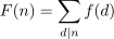
where the sum is taken over the positive divisors of n. Then the values of f(n) can be recovered from the
values of F(n):
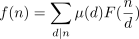
where again the sum is taken over the positive divisors of n.
When f(n)= 1, then F(n)= d(n). Thus, if you sum  (d)d(n/d)
d of n, you should
always get 1.
f1(n) == reduce(+,[moebiusMu(d) * numberOfDivisors(quo(n,d)) for d in divisors(n)])
f1(200)
Compiling function f1 with type PositiveInteger -> Integer
f1(846)
PositiveInteger Similarly, when f(n)= n, then F(n)= . Thus, if you sum  (n)
 (d)
 (n/d)
d of n, you should always get n.
f2(n) == reduce(+,[moebiusMu(d) * sumOfDivisors(quo(n,d)) for d in divisors(n)])
f2(200)
Compiling function f2 with type PositiveInteger -> Integer
f2(846)
The Möbius inversion formula is derived from the multiplication of formal Dirichlet series. A Dirichlet series is an infinite series of the form

When

then  Recall that the Riemann
 function is defined by

where the product is taken over the set of (positive) primes. Thus,

Now if  then

Thus,

and  .
The Fibonacci numbers are defined by F(1)= F(2)= 1 and F(n)= F(n-1)+ F(n-2) for n = 3,4, .... The
operation fibonacci computes the  Fibonacci number.
fibonacci(25)
[fibonacci(n) for n in 1..15]
List(Integer) Fibonacci numbers can also be expressed as sums of binomial coefficients.
fib(n) == reduce(+,[binomial(n-1-k,k) for k in 0..quo(n-1,2)])
fib(25)
Compiling function fib with type PositiveInteger -> Integer
[fib(n) for n in 1..15]
Quadratic symbols can be computed with the operations legendre and jacobi. The Legendre symbol  is
defined for integers
a and p with p an odd prime number. By definition,  , when
a is a square (mod p),
 , when
a is not a square (mod p), and  , when
a is divisible by p. You compute  via the
command
legendre(a,p).
legendre(3,5)
legendre(23,691)
Integer The Jacobi symbol  is the usual extension of the Legendre symbol, where
n is an arbitrary
integer. The most important property of the Jacobi symbol is the following: if K is a quadratic field with
discriminant d and quadratic character  , then

(n)= (d/n). Thus, you can use the Jacobi symbol to
compute, say, the class numbers of imaginary quadratic fields from a standard class number formula.
This function computes the class number of the imaginary quadratic field with discriminant
d.
h(d) == quo(reduce(+, [jacobi(d,k) for k in 1..quo(-d, 2)]), 2 - jacobi(d,2))
h(-163)
Compiling function h with type Integer -> Integer
h(-499)
h(-1832)
A kernel is a symbolic function application (such as sin(x + y)) or a symbol (such as x). More precisely, a
non-symbol kernel over a set S is an operator applied to a given list of arguments from S. The operator has
type BasicOperator (see ‘BasicOperator’ on page 695) and the kernel object is usually part of an
expression object (see ‘Expression’ on page 847).
Kernels are created implicitly for you when you create expressions.
x :: Expression Integer
Expression(Integer) You can directly create a “symbol” kernel by using the kernel operation.
kernel x
Kernel(Expression(Integer)) This expression has two different kernels.
sin(x) + cos(x)
Expression(Integer) The operator kernels returns a list of the kernels in an object of type Expression.
kernels %
List(Kernel(Expression(Integer))) This expression also has two different kernels.
sin(x)^2 + sin(x) + cos(x)
Expression(Integer) The sin(x) kernel is used twice.
kernels %
List(Kernel(Expression(Integer))) An expression need not contain any kernels.
kernels(1 :: Expression Integer)
List(Kernel(Expression(Integer))) If one or more kernels are present, one of them is designated the main kernel.
mainKernel(cos(x) + tan(x))
Union(Kernel(Expression(Integer)), ...) Kernels can be nested. Use height to determine the nesting depth.
height kernel x
PositiveInteger This has height 2 because the x has height 1 and then we apply an operator to that.
height mainKernel(sin x)
height mainKernel(sin cos x)
height mainKernel(sin cos (tan x + sin x))
PositiveInteger Use the operator operation to extract the operator component of the kernel. The operator has type BasicOperator.
operator mainKernel(sin cos (tan x + sin x))
BasicOperator Use the name operation to extract the name of the operator component of the kernel. The name has type Symbol. This is really just a shortcut for a two-step process of extracting the operator and then calling name on the operator.
name mainKernel(sin cos (tan x + sin x))
Symbol FriCAS knows about functions such as sin, cos and so on and can make kernels and then expressions
using them. To create a kernel and expression using an arbitrary operator, use operator. Now f can be used
to create symbolic function applications.
f := operator ’f
e := f(x, y, 10)
Expression(Integer) Use the is? operation to learn if the operator component of a kernel is equal to a given operator.
is?(e, f)
Boolean You can also use a symbol or a string as the second argument to is?.
is?(e, ’f)
Boolean Use the argument operation to get a list containing the argument component of a kernel.
argument mainKernel e
Conceptually, an object of type Expression can be thought of as a quotient of multivariate polynomials, where the “variables” are kernels. The arguments of the kernels are again expressions and so the structure recurses. See ‘Expression’ on page 847 for examples of using kernels to take apart expression objects.
The domain KeyedAccessFile(S) provides files which can be used as associative tables. Data values are stored in these files and can be retrieved according to their keys. The keys must be strings so this type behaves very much like the StringTable(S) domain. The difference is that keyed access files reside in secondary storage while string tables are kept in memory. For more information on table-oriented operations, see the description of Table.
Before a keyed access file can be used, it must first be opened. A new file can be created by opening it for output.
ey: KeyedAccessFile(Integer) := open("/tmp/editor.year", "output")
KeyedAccessFile(Integer) Just as for vectors, tables or lists, values are saved in a keyed access file by setting elements.
ey."Char" := 1986
ey."Caviness" := 1985
ey."Fitch" := 1984
PositiveInteger Values are retrieved using application, in any of its syntactic forms.
ey."Char"
ey("Char")
ey "Char"
PositiveInteger Attempting to retrieve a non-existent element in this way causes an error. If it is not known whether a key exists, you should use the search operation.
search("Char", ey)
search("Smith", ey)
Union("failed", ...) When an entry is no longer needed, it can be removed from the file.
remove!("Char", ey)
Union(Integer, ...) The keys operation returns a list of all the keys for a given file.
keys ey
List(String) The # operation gives the number of entries.
#ey
The table view of keyed access files provides safe operations. That is, if the FriCAS program is terminated between file operations, the file is left in a consistent, current state. This means, however, that the operations are somewhat costly. For example, after each update the file is closed. Here we add several more items to the file, then check its contents.
KE := Record(key: String, entry: Integer)
reopen!(ey, "output")
KeyedAccessFile(Integer) If many items are to be added to a file at the same time, then it is more efficient to use the write! operation.
write!(ey, ["van Hulzen", 1983]$KE)
Record(key: String, entry: Integer)
write!(ey, ["Calmet", 1982]$KE)
Record(key: String, entry: Integer)
write!(ey, ["Wang", 1981]$KE)
Record(key: String, entry: Integer)
close! ey
KeyedAccessFile(Integer) The read! operation is also available from the file view, but it returns elements in a random order. It is generally clearer and more efficient to use the keys operation and to extract elements by key.
keys ey
members ey
)system rm -r /tmp/editor.year
For more information on related topics, see ‘File’ on page 876, ‘TextFile’ on page 1338, and ‘Library’ on page 1031. Issue the system command )show KeyedAccessFile to display the full list of operations defined by KeyedAccessFile.
The LazardSetSolvingPackage package constructor solves polynomial systems by means of Lazard triangular sets. However one condition is relaxed: Regular triangular sets whose saturated ideals have positive dimension are not necessarily normalized.
The decompositions are computed in two steps. First the algorithm of Moreno Maza (implemented in the RegularTriangularSet domain constructor) is called. Then the resulting decompositions are converted into lists of square-free regular triangular sets and the redundant components are removed. Moreover, zero-dimensional regular triangular sets are normalized.
Note that the way of understanding triangular decompositions is detailed in the example of the RegularTriangularSet constructor.
The LazardSetSolvingPackage constructor takes six arguments. The first one, R, is the coefficient ring of
the polynomials; it must belong to the category GcdDomain. The second one, E, is the exponent monoid of
the polynomials; it must belong to the category OrderedAbelianMonoidSup. The third one, V, is the
ordered set of variables; it must belong to the category OrderedSet. The fourth one is the polynomial ring; it
must belong to the category RecursivePolynomialCategory(R,E,V). The fifth one is a domain
of the category RegularTriangularSetCategory(R,E,V,P) and the last one is a domain of
the category SquareFreeRegularTriangularSetCategory(R,E,V,P). The abbreviation for
LazardSetSolvingPackage is LAZM3PK.
N.B. For the purpose of solving zero-dimensional algebraic systems, see also LexTriangularPackage and
ZeroDimensionalSolvePackage. These packages are easier to call than LAZM3PK. Moreover, the
ZeroDimensionalSolvePackage package provides operations to compute either the complex roots or the
real roots.
We illustrate now the use of the LazardSetSolvingPackage package constructor with two examples (Butcher and Vermeer).
Define the coefficient ring.
R := Integer
Define the list of variables,
ls : List Symbol := [b1,x,y,z,t,v,u,w]
and make it an ordered set;
V := OVAR(ls)
then define the exponent monoid.
E := IndexedExponents V
Define the polynomial ring.
P := NSMP(R, V)
Let the variables be polynomial.
b1: P := ’b1
NewSparseMultivariatePolynomial(Integer, OrderedVariableList([b1, x, y, z, t, v, u, w]))
x: P := ’x
NewSparseMultivariatePolynomial(Integer, OrderedVariableList([b1, x, y, z, t, v, u, w]))
y: P := ’y
NewSparseMultivariatePolynomial(Integer, OrderedVariableList([b1, x, y, z, t, v, u, w]))
z: P := ’z
NewSparseMultivariatePolynomial(Integer, OrderedVariableList([b1, x, y, z, t, v, u, w]))
t: P := ’t
NewSparseMultivariatePolynomial(Integer, OrderedVariableList([b1, x, y, z, t, v, u, w]))
u: P := ’u
NewSparseMultivariatePolynomial(Integer, OrderedVariableList([b1, x, y, z, t, v, u, w]))
v: P := ’v
NewSparseMultivariatePolynomial(Integer, OrderedVariableList([b1, x, y, z, t, v, u, w]))
w: P := ’w
NewSparseMultivariatePolynomial(Integer, OrderedVariableList([b1, x, y, z, t, v, u, w]))
Now call the RegularTriangularSet domain constructor.
T := REGSET(R,E,V,P)
Define a polynomial system (the Butcher example).
p0 := b1 + y + z - t - w
NewSparseMultivariatePolynomial(Integer, OrderedVariableList([b1, x, y, z, t, v, u, w]))
p1 := 2*z*u + 2*y*v + 2*t*w - 2*w^2 - w - 1
NewSparseMultivariatePolynomial(Integer, OrderedVariableList([b1, x, y, z, t, v, u, w]))
p2 := 3*z*u^2 + 3*y*v^2 - 3*t*w^2 + 3*w^3 + 3*w^2 - t + 4*w
NewSparseMultivariatePolynomial(Integer, OrderedVariableList([b1, x, y, z, t, v, u, w]))
p3 := 6*x*z*v - 6*t*w^2 + 6*w^3 - 3*t*w + 6*w^2 - t + 4*w
NewSparseMultivariatePolynomial(Integer, OrderedVariableList([b1, x, y, z, t, v, u, w]))
p4 := 4*z*u^3+ 4*y*v^3+ 4*t*w^3- 4*w^4 - 6*w^3+ 4*t*w- 10*w^2- w- 1
NewSparseMultivariatePolynomial(Integer, OrderedVariableList([b1, x, y, z, t, v, u, w]))
p5 := 8*x*z*u*v +8*t*w^3 -8*w^4 +4*t*w^2 -12*w^3 +4*t*w -14*w^2 -3*w -1
NewSparseMultivariatePolynomial(Integer, OrderedVariableList([b1, x, y, z, t, v, u, w]))
p6 := 12*x*z*v^2+12*t*w^3 -12*w^4 +12*t*w^2 -18*w^3 +8*t*w -14*w^2 -w -1
NewSparseMultivariatePolynomial(Integer, OrderedVariableList([b1, x, y, z, t, v, u, w]))
p7 := -24*t*w^3 + 24*w^4 - 24*t*w^2 + 36*w^3 - 8*t*w + 26*w^2 + 7*w + 1
NewSparseMultivariatePolynomial(Integer, OrderedVariableList([b1, x, y, z, t, v, u, w]))
lp := [p0, p1, p2, p3, p4, p5, p6, p7]
List(NewSparseMultivariatePolynomial(Integer, OrderedVariableList([b1, x, y, z, t, v, u, w])))
First of all, let us solve this system in the sense of Lazard by means of the REGSET constructor:
lts := zeroSetSplit(lp,false)$T
We can get the dimensions of each component of a decomposition as follows.
[coHeight(ts) for ts in lts]
The first five sets have a simple shape. However, the last one, which has dimension zero, can be simplified by using Lazard triangular sets.
Thus we call the SquareFreeRegularTriangularSet domain constructor,
ST := SREGSET(R,E,V,P)
and set the LAZM3PK package constructor to our situation.
pack := LAZM3PK(R,E,V,P,T,ST)
We are ready to solve the system by means of Lazard triangular sets:
zeroSetSplit(lp,false)$pack
We see the sixth triangular set is nicer now: each one of its polynomials has a constant initial.
We follow with the Vermeer example. The ordering is the usual one for this system.
Define the polynomial system.
f0 := (w - v) ^ 2 + (u - t) ^ 2 - 1
NewSparseMultivariatePolynomial(Integer, OrderedVariableList([b1, x, y, z, t, v, u, w]))
f1 := t ^ 2 - v ^ 3
NewSparseMultivariatePolynomial(Integer, OrderedVariableList([b1, x, y, z, t, v, u, w]))
f2 := 2 * t * (w - v) + 3 * v ^ 2 * (u - t)
NewSparseMultivariatePolynomial(Integer, OrderedVariableList([b1, x, y, z, t, v, u, w]))
f3 := (3 * z * v ^ 2 - 1) * (2 * z * t - 1)
NewSparseMultivariatePolynomial(Integer, OrderedVariableList([b1, x, y, z, t, v, u, w]))
lf := [f0, f1, f2, f3]
List(NewSparseMultivariatePolynomial(Integer, OrderedVariableList([b1, x, y, z, t, v, u, w])))
First of all, let us solve this system in the sense of Kalkbrener by means of the REGSET constructor:
zeroSetSplit(lf,true)$T
We have obtained one regular chain (i.e. regular triangular set) with dimension 1. This set is in fact a characterist set of the (radical of) of the ideal generated by the input system lf. Thus we have only the generic points of the variety associated with lf (for the elimination ordering given by ls).
So let us get now a full description of this variety. Hence, we solve this system in the sense of Lazard by means of the REGSET constructor:
zeroSetSplit(lf,false)$T
We retrieve our regular chain of dimension 1 and we get three regular chains of dimension 0 corresponding to the degenerate cases. We want now to simplify these zero-dimensional regular chains by using Lazard triangular sets. Moreover, this will allow us to prove that the above decomposition has no redundant component. N.B. Generally, decompositions computed by the REGSET constructor do not have redundant components. However, to be sure that no redundant component occurs one needs to use the SREGSET or LAZM3PK constructors.
So let us solve the input system in the sense of Lazard by means of the LAZM3PK constructor:
zeroSetSplit(lf,false)$pack
List(SquareFreeRegularTriangularSet(Integer, IndexedExponents(OrderedVariableList([b1, x, y, z, t, v, u, w])), OrderedVariableList([b1, x, y, z, t, v, u, w]), NewSparseMultivariatePolynomial(Integer, OrderedVariableList([b1, x, y, z, t, v, u, w])))) Due to square-free factorization, we obtained now four zero-dimensional regular chains. Moreover, each of them is normalized (the initials are constant). Note that these zero-dimensional components may be investigated further with the ZeroDimensionalSolvePackage package constructor.
The LexTriangularPackage package constructor provides an implementation of the lexTriangular algorithm (D. Lazard ”Solving Zero-dimensional Algebraic Systems”, J. of Symbol. Comput., 1992). This algorithm decomposes a zero-dimensional variety into zero-sets of regular triangular sets. Thus the input system must have a finite number of complex solutions. Moreover, this system needs to be a lexicographical Groebner basis.
This package takes two arguments: the coefficient-ring R of the polynomials, which must be a GcdDomain and their set of variables given by ls a List Symbol. The type of the input polynomials must be NewSparseMultivariatePolynomial(R,V) where V is OrderedVariableList(ls). The abbreviation for LexTriangularPackage is LEXTRIPK. The main operations are lexTriangular and squareFreeLexTriangular. The latter provides decompositions by means of square-free regular triangular sets, built with the SREGSET constructor, whereas the former uses the REGSET constructor. Note that these constructors also implement another algorithm for solving algebraic systems by means of regular triangular sets; in that case no computations of Groebner bases are needed and the input system may have any dimension (i.e. it may have an infinite number of solutions).
The implementation of the lexTriangular algorithm provided in the LexTriangularPackage constructor differs from that reported in ”Computations of gcd over algebraic towers of simple extensions” by M. Moreno Maza and R. Rioboo (in proceedings of AAECC11, Paris, 1995). Indeed, the squareFreeLexTriangular operation removes all multiplicities of the solutions (i.e. the computed solutions are pairwise different) and the lexTriangular operation may keep some multiplicities; this latter operation runs generally faster than the former.
The interest of the lexTriangular algorithm is due to the following experimental remark. For some examples, a triangular decomposition of a zero-dimensional variety can be computed faster via a lexicographical Groebner basis computation than by using a direct method (like that of SREGSET and REGSET). This happens typically when the total degree of the system relies essentially on its smallest variable (like in the Katsura systems). When this is not the case, the direct method may give better timings (like in the Rose system).
Of course, the direct method can also be applied to a lexicographical Groebner basis. However, the lexTriangular algorithm takes advantage of the structure of this basis and avoids many unnecessary computations which are performed by the direct method.
For this purpose of solving algebraic systems with a finite number of solutions, see also the ZeroDimensionalSolvePackage. It allows one to use both strategies (the lexTriangular algorithm and the direct method) for computing either the complex or real roots of a system.
Note that the way of understanding triangular decompositions is detailed in the example of the RegularTriangularSet constructor.
Since the LEXTRIPK package constructor is limited to zero-dimensional systems, it provides a zeroDimensional? operation to check whether this requirement holds. There is also a groebner operation to compute the lexicographical Groebner basis of a set of polynomials with type NewSparseMultivariatePolynomial(R,V). The elimination ordering is that given by ls (the greatest variable being the first element of ls). This basis is computed by the FLGM algorithm (Faugere et al. ”Efficient Computation of Zero-Dimensional Groebner Bases by Change of Ordering” , J. of Symbol. Comput., 1993) implemented in the LinGroebnerPackage package constructor. Once a lexicographical Groebner basis is computed, then one can call the operations lexTriangular and squareFreeLexTriangular. Note that these operations admit an optional argument to produce normalized triangular sets. There is also a zeroSetSplit operation which does all the job from the input system; an error is produced if this system is not zero-dimensional.
Let us illustrate the facilities of the LEXTRIPK constructor by a famous example, the cyclic-6 root system. Define the coefficient ring.
R := Integer
Type Define the list of variables,
ls : List Symbol := [a,b,c,d,e,f]
List(Symbol) and make it an ordered set.
V := OVAR(ls)
Type Define the polynomial ring.
P := NSMP(R, V)
Type Define the polynomials.
p1: P := a*b*c*d*e*f - 1
NewSparseMultivariatePolynomial(Integer, OrderedVariableList([a, b, c, d, e, f]))
p2: P := a*b*c*d*e +a*b*c*d*f +a*b*c*e*f +a*b*d*e*f +a*c*d*e*f +b*c*d*e*f
NewSparseMultivariatePolynomial(Integer, OrderedVariableList([a, b, c, d, e, f]))
p3: P := a*b*c*d + a*b*c*f + a*b*e*f + a*d*e*f + b*c*d*e + c*d*e*f
NewSparseMultivariatePolynomial(Integer, OrderedVariableList([a, b, c, d, e, f]))
p4: P := a*b*c + a*b*f + a*e*f + b*c*d + c*d*e + d*e*f
NewSparseMultivariatePolynomial(Integer, OrderedVariableList([a, b, c, d, e, f]))
p5: P := a*b + a*f + b*c + c*d + d*e + e*f
NewSparseMultivariatePolynomial(Integer, OrderedVariableList([a, b, c, d, e, f]))
p6: P := a + b + c + d + e + f
NewSparseMultivariatePolynomial(Integer, OrderedVariableList([a, b, c, d, e, f]))
lp := [p1, p2, p3, p4, p5, p6]
List(NewSparseMultivariatePolynomial(Integer, OrderedVariableList([a, b, c, d, e, f]))) Now call LEXTRIPK .
lextripack := LEXTRIPK(R,ls)
Type Compute the lexicographical Groebner basis of the system. This may take between 5 minutes and one hour, depending on your machine.
lg := groebner(lp)$lextripack;
List(NewSparseMultivariatePolynomial(Integer, OrderedVariableList([a, b, c, d, e, f]))) Apply lexTriangular to compute a decomposition into regular triangular sets. This should not take more than 5 seconds.
lexTriangular(lg,false)$lextripack
List(RegularChain(Integer, [a, b, c, d, e, f])) Note that the first set of the decomposition is normalized (all initials are integer numbers) but not the second one (normalized triangular sets are defined in the description of the NormalizedTriangularSetCategory constructor). So apply now lexTriangular to produce normalized triangular sets.
lts := lexTriangular(lg,true)$lextripack
List(RegularChain(Integer, [a, b, c, d, e, f])) We check that all initials are constant.
[[init(p) for p in (ts :: List(P))] for ts in lts]
List(List(NewSparseMultivariatePolynomial(Integer, OrderedVariableList([a, b, c, d, e, f])))) Note that each triangular set in lts is a lexicographical Groebner basis. Recall that a point belongs to the variety associated with lp if and only if it belongs to that associated with one triangular set ts in lts.
By running the squareFreeLexTriangular operation, we retrieve the above decomposition.
squareFreeLexTriangular(lg,true)$lextripack
List(SquareFreeRegularTriangularSet(Integer, IndexedExponents(OrderedVariableList([a, b, c, d, e, f])), OrderedVariableList([a, b, c, d, e, f]), NewSparseMultivariatePolynomial(Integer, OrderedVariableList([a, b, c, d, e, f])))) Thus the solutions given by lts are pairwise different. We count them as follows.
reduce(+,[degree(ts) for ts in lts])
We can investigate the triangular decomposition lts by using the ZeroDimensionalSolvePackage. This requires adding an extra variable (smaller than the others) as follows.
ls2 : List Symbol := concat(ls,new()$Symbol)
Then we call the package.
zdpack := ZDSOLVE(R,ls,ls2)
We compute a univariate representation of the variety associated with the input system as follows.
concat [univariateSolve(ts)$zdpack for ts in lts];
List(Record(complexRoots: SparseUnivariatePolynomial(Integer), coordinates: List(Polynomial(Integer)))) Since the univariateSolve operation may split a regular set, it returns a list. This explains the use of concat.
Look at the last item of the result. It consists of two parts. For any complex root ? of the univariate polynomial in the first part, we get a tuple of univariate polynomials (in a, ..., f respectively) by replacing %A by ? in the second part. Each of these tuples t describes a point of the variety associated with lp by equaling to zero the polynomials in t.
Note that the way of reading these univariate representations is explained also in the example illustrating the ZeroDimensionalSolvePackage constructor.
Now, we compute the points of the variety with real coordinates.
concat [realSolve(ts)$zdpack for ts in lts];
List(List(RealClosure(Fraction(Integer)))) We obtain 24 points given by lists of elements in the RealClosure of Fraction of R. In each list, the first value corresponds to the indeterminate f, the second to e and so on. See ZeroDimensionalSolvePackage to learn more about the realSolve operation.
The Library domain provides a simple way to store FriCAS values in a file. This domain is similar to KeyedAccessFile but fewer declarations are needed and items of different types can be saved together in the same file.
To create a library, you supply a file name.
stuff := library "/tmp/Neat.stuff"
Library Now values can be saved by key in the file. The keys should be mnemonic, just as the field names are for records. They can be given either as strings or symbols.
stuff.int := 32^2
stuff."poly" := x^2 + 1
stuff.str := "Hello"
String You obtain the set of available keys using the keys operation.
keys stuff
List(String) You extract values by giving the desired key in this way.
stuff.poly
stuff("poly")
Polynomial(Integer) When the file is no longer needed, you should remove it from the file system.
)system rm -rf /tmp/Neat.stuff
For more information on related topics, see ‘File’ on page 876, ‘TextFile’ on page 1338, and ‘KeyedAccessFile’ on page 997. Issue the system command )show Library to display the full list of operations defined by Library.
This example is in just two variables
a: Symbol := ’a
b: Symbol := ’b
Declarations of domains
coef := Fraction(Integer)
group := LieExponentials(Symbol, coef, 3)
lpoly := LiePolynomial(Symbol, coef)
poly := XPBWPolynomial(Symbol, coef)
Calculations
ea := exp(a::lpoly)$group
LieExponentials(Symbol, Fraction(Integer), 3)
eb := exp(b::lpoly)$group
LieExponentials(Symbol, Fraction(Integer), 3)
g: group := ea*eb
LieExponentials(Symbol, Fraction(Integer), 3)
g :: poly
XPBWPolynomial(Symbol, Fraction(Integer))
log(g)$group
LiePolynomial(Symbol, Fraction(Integer))
g1: group := inv(g)
LieExponentials(Symbol, Fraction(Integer), 3)
g*g1
LieExponentials(Symbol, Fraction(Integer), 3)
Declaration of domains
RN := Fraction Integer
Lpoly := LiePolynomial(Symbol,RN)
Dpoly := XDPOLY(Symbol,RN)
Lword := LyndonWord Symbol
Initialisation
a:Symbol := ’a
b:Symbol := ’b
c:Symbol := ’c
aa: Lpoly := a
LiePolynomial(Symbol, Fraction(Integer))
bb: Lpoly := b
LiePolynomial(Symbol, Fraction(Integer))
cc: Lpoly := c
LiePolynomial(Symbol, Fraction(Integer))
p : Lpoly := [aa,bb]
LiePolynomial(Symbol, Fraction(Integer))
q : Lpoly := [p,bb]
LiePolynomial(Symbol, Fraction(Integer)) All the Lyndon words of order 4
liste : List Lword := LyndonWordsList([a,b], 4)
r: Lpoly := p + q + 3*LiePoly(liste.4)$Lpoly
LiePolynomial(Symbol, Fraction(Integer))
s:Lpoly := [p,r]
LiePolynomial(Symbol, Fraction(Integer))
t:Lpoly := s + 2*LiePoly(liste.3) - 5*LiePoly(liste.5)
LiePolynomial(Symbol, Fraction(Integer))
degree t
mirror t
LiePolynomial(Symbol, Fraction(Integer))
Jacobi Relation
Jacobi(p: Lpoly, q: Lpoly, r: Lpoly): Lpoly == [[p,q]$Lpoly, r] + [[q,r]$Lpoly, p] + [[r,p]$Lpoly, q]
Function declaration Jacobi : (LiePolynomial(Symbol,Fraction(Integer)), LiePolynomial(Symbol,Fraction(Integer)), LiePolynomial(Symbol,Fraction( Integer))) -> LiePolynomial(Symbol,Fraction(Integer)) has been added to workspace.
Tests
test: Lpoly := Jacobi(a,b,b)
Compiling function Jacobi with type (LiePolynomial(Symbol,Fraction(Integer)), LiePolynomial(Symbol,Fraction(Integer)), LiePolynomial(Symbol,Fraction( Integer))) -> LiePolynomial(Symbol,Fraction(Integer))
LiePolynomial(Symbol, Fraction(Integer))
test: Lpoly := Jacobi(p,q,r)
LiePolynomial(Symbol, Fraction(Integer))
test: Lpoly := Jacobi(r,s,t)
LiePolynomial(Symbol, Fraction(Integer))
Evaluation
eval(p, a, p)$Lpoly
LiePolynomial(Symbol, Fraction(Integer))
eval(p, [a,b], [2*bb, 3*aa])$Lpoly
LiePolynomial(Symbol, Fraction(Integer))
r: Lpoly := [p,c]
LiePolynomial(Symbol, Fraction(Integer))
r1: Lpoly := eval(r, [a,b,c], [bb, cc, aa])$Lpoly
LiePolynomial(Symbol, Fraction(Integer))
r2: Lpoly := eval(r, [a,b,c], [cc, aa, bb])$Lpoly
LiePolynomial(Symbol, Fraction(Integer))
r + r1 + r2
LiePolynomial(Symbol, Fraction(Integer))
LinearOrdinaryDifferentialOperator(A, diff) is the domain of linear ordinary differential
operators with coefficients in a ring A with a given derivation. Issue the system command
)show LinearOrdinaryDifferentialOperator to display the full list of operations defined by
LinearOrdinaryDifferentialOperator.
Problem: Find the first few coefficients of exp(x)/x^i of Dop( where
 )
Dop := D^3 + G/x^2 * D + H/x^3 - 1 phi := sum(s[i]*exp(x)/x^i, i = 0..)
Solution: Define the differential.
Dx: LODO(EXPR INT, f +-> D(f, x))
Dx := D()
LinearOrdinaryDifferentialOperator(Expression(Integer), theMap(anonymousFunction)) Now define the differential operator Dop.
Dop:= Dx^3 + G/x^2*Dx + H/x^3 - 1
LinearOrdinaryDifferentialOperator(Expression(Integer), theMap(anonymousFunction)) The first  coefficients can be obtained in the following
way.
firstCoefficients(n) == phi := reduce(+, [subscript(s,[i])*exp(x)/x^i for i in 0..n]) phi1 := retract((Dop(phi) * x^(n+3) / exp x))@Polynomial(Integer) phi2 := phi1 :: UnivariatePolynomial(x, Polynomial Integer) sys := [coefficient(phi2, (n+3-i)::NNI) for i in 2..n+1] solve(sys, [subscript(s,[i]) for i in 1..n])
Evaluate this function for several values of n.
firstCoefficients(3)
Compiling function firstCoefficients with type PositiveInteger -> List(List( Equation(Fraction(Polynomial(Integer)))))
Compiling function G27 with type Integer -> Boolean
List(List(Equation(Fraction(Polynomial(Integer)))))
firstCoefficients(4)
List(List(Equation(Fraction(Polynomial(Integer)))))
firstCoefficients(7)
List(List(Equation(Fraction(Polynomial(Integer)))))
LinearOrdinaryDifferentialOperator1(A) is the domain of linear ordinary differential operators with
coefficients in the differential ring A. Issue the system command )show LinearOrdinaryDifferentialOperator1
to display the full list of operations defined by LinearOrdinaryDifferentialOperator1.
This example shows differential operators with rational function coefficients. In this case operator multiplication is non-commutative and, since the coefficients form a field, an operator division algorithm exists.
We begin by defining RFZ to be the rational functions in x with integer coefficients and Dx to be the
differential operator for d/dx.
RFZ := Fraction UnivariatePolynomial(’x, Integer)
x : RFZ := ’x
Fraction(UnivariatePolynomial(x, Integer))
Dx : LODO1 RFZ := D()
LinearOrdinaryDifferentialOperator1(Fraction(UnivariatePolynomial(x, Integer))) Operators are created using the usual arithmetic operations.
b : LODO1 RFZ := 3*x^2*Dx^2 + 2*Dx + 1/x
LinearOrdinaryDifferentialOperator1(Fraction(UnivariatePolynomial(x, Integer)))
a : LODO1 RFZ := b*(5*x*Dx + 7)
LinearOrdinaryDifferentialOperator1(Fraction(UnivariatePolynomial(x, Integer))) Operator multiplication corresponds to functional composition.
p := x^2 + 1/x^2
Fraction(UnivariatePolynomial(x, Integer)) Since operator coefficients depend on x, the multiplication is not commutative.
(a*b - b*a) p
Fraction(UnivariatePolynomial(x, Integer))
When the coefficients of operator polynomials come from a field, as in this case, it is possible to define operator division. Division on the left and division on the right yield different results when the multiplication is non-commutative.
The results of leftDivide and rightDivide are quotient-remainder pairs satisfying: leftDivide(a,b)= [q, r] such that a = b*q + r rightDivide(a,b)= [q, r] such that a = q*b + r
In both cases, the degree of the remainder, r, is less than the degree of b.
ld := leftDivide(a,b)
a = b * ld.quotient + ld.remainder
Equation(LinearOrdinaryDifferentialOperator1(Fraction(UnivariatePolynomial(x, Integer)))) The operations of left and right division are so-called because the quotient is obtained by
dividing a on that side by b.
rd := rightDivide(a,b)
a = rd.quotient * b + rd.remainder
Equation(LinearOrdinaryDifferentialOperator1(Fraction(UnivariatePolynomial(x, Integer))))
Operations rightQuotient and rightRemainder are available if only one of the quotient or remainder is of interest to you. This is the quotient from right division.
rightQuotient(a,b)
LinearOrdinaryDifferentialOperator1(Fraction(UnivariatePolynomial(x, Integer))) This is the remainder from right division. The corresponding “left” functions leftQuotient and leftRemainder are also available.
rightRemainder(a,b)
LinearOrdinaryDifferentialOperator1(Fraction(UnivariatePolynomial(x, Integer)))
For exact division, the operations leftExactQuotient and rightExactQuotient are supplied. These return the
quotient but only if the remainder is zero. The call rightExactQuotient(a,b) would yield an
error.
leftExactQuotient(a,b)
Union(LinearOrdinaryDifferentialOperator1(Fraction(UnivariatePolynomial(x, Integer))), ...)
The division operations allow the computation of left and right greatest common divisors (leftGcd and rightGcd) via remainder sequences, and consequently the computation of left and right least common multiples (rightLcm and leftLcm).
e := leftGcd(a,b)
LinearOrdinaryDifferentialOperator1(Fraction(UnivariatePolynomial(x, Integer))) Note that a greatest common divisor doesn’t necessarily
divide a and b on both sides. Here the left greatest common divisor does not divide a on the
right.
leftRemainder(a, e)
LinearOrdinaryDifferentialOperator1(Fraction(UnivariatePolynomial(x, Integer)))
rightRemainder(a, e)
LinearOrdinaryDifferentialOperator1(Fraction(UnivariatePolynomial(x, Integer)))
Similarly, a least common multiple is not necessarily divisible from both sides.
f := rightLcm(a,b)
LinearOrdinaryDifferentialOperator1(Fraction(UnivariatePolynomial(x, Integer)))
rightRemainder(f, b)
LinearOrdinaryDifferentialOperator1(Fraction(UnivariatePolynomial(x, Integer)))
leftRemainder(f, b)
LinearOrdinaryDifferentialOperator1(Fraction(UnivariatePolynomial(x, Integer)))
LinearOrdinaryDifferentialOperator2(A, M) is the domain of linear ordinary differential operators with
coefficients in the differential ring A and operating on M, an A-module. This includes the cases of operators
which are polynomials in D acting upon scalar or vector expressions of a single variable. The coefficients of the
operator polynomials can be integers, rational functions, matrices or elements of other domains. Issue the
system command )show LinearOrdinaryDifferentialOperator2 to display the full list of operations
defined by LinearOrdinaryDifferentialOperator2.
This example shows differential operators with rational number coefficients operating on univariate polynomials.
We begin by making type assignments so we can conveniently refer to univariate polynomials in x over the
rationals.
Q := Fraction Integer
PQ := UnivariatePolynomial(’x, Q)
x: PQ := ’x
UnivariatePolynomial(x, Fraction(Integer)) Now we assign Dx to be the differential operator D corresponding to
d/dx.
Dx: LODO2(Q, PQ) := D()
LinearOrdinaryDifferentialOperator2(Fraction(Integer), UnivariatePolynomial(x, Fraction(Integer))) New operators are created as polynomials in
D().
a := Dx + 1
LinearOrdinaryDifferentialOperator2(Fraction(Integer), UnivariatePolynomial(x, Fraction(Integer)))
b := a + 1/2*Dx^2 - 1/2
LinearOrdinaryDifferentialOperator2(Fraction(Integer), UnivariatePolynomial(x, Fraction(Integer))) To apply the operator a to the value p the usual function call
syntax is used.
p := 4*x^2 + 2/3
UnivariatePolynomial(x, Fraction(Integer))
a p
UnivariatePolynomial(x, Fraction(Integer)) Operator multiplication is defined by the identity (a*b)p = a(b(p))
(a * b) p = a b p
Equation(UnivariatePolynomial(x, Fraction(Integer))) Exponentiation follows from multiplication.
c := (1/9)*b*(a + b)^2
LinearOrdinaryDifferentialOperator2(Fraction(Integer), UnivariatePolynomial(x, Fraction(Integer))) Finally, note that operator expressions may be applied directly.
(a^2 - 3/4*b + c) (p + 1)
UnivariatePolynomial(x, Fraction(Integer))
This is another example of linear ordinary differential operators with non-commutative multiplication. Unlike the rational function case, the differential ring of square matrices (of a given dimension) with univariate polynomial entries does not form a field. Thus the number of operations available is more limited.
In this section, the operators have three by three matrix coefficients with polynomial entries.
PZ := UnivariatePolynomial(x,Integer)
x:PZ := ’x
UnivariatePolynomial(x, Integer)
Mat := SquareMatrix(3,PZ)
Type The operators act on the vectors considered as a Mat-module.
Vect := DPMM(3, PZ, Mat, PZ);
Modo := LODO2(Mat, Vect);
Type The matrix m is used as a coefficient and the vectors p and q are operated upon.
m:Mat := matrix [[x^2,1,0],[1,x^4,0],[0,0,4*x^2]]
SquareMatrix(3, UnivariatePolynomial(x, Integer))
p:Vect := directProduct [3*x^2+1,2*x,7*x^3+2*x]
q: Vect := m * p
DirectProductMatrixModule(3, UnivariatePolynomial(x, Integer), SquareMatrix(3, UnivariatePolynomial(x, Integer)), UnivariatePolynomial(x, Integer)) Now form a few operators.
Dx : Modo := D()
a : Modo := Dx + m
b : Modo := m*Dx + 1
c := a*b
LinearOrdinaryDifferentialOperator2(SquareMatrix(3, UnivariatePolynomial(x, Integer)), DirectProductMatrixModule(3, UnivariatePolynomial(x, Integer), SquareMatrix(3, UnivariatePolynomial(x, Integer)), UnivariatePolynomial(x, Integer))) These operators can be applied to vector values.
a p
b p
(a + b + c) (p + q)
A list is a finite collection of elements in a specified order that can contain duplicates. A list is a convenient structure to work with because it is easy to add or remove elements and the length need not be constant. There are many different kinds of lists in FriCAS, but the default types (and those used most often) are created by the List constructor. For example, there are objects of type List Integer, List Float and List Polynomial Fraction Integer. Indeed, you can even have List List List Boolean (that is, lists of lists of lists of Boolean values). You can have lists of any type of FriCAS object.
The easiest way to create a list with, for example, the elements 2, 4, 5, 6 is to enclose the elements with square
brackets and separate the elements with commas. The spaces after the commas are optional, but they do
improve the readability.
[2, 4, 5, 6]
List(PositiveInteger) To create a list with the single element 1, you can use either [1] or the operation
list.
[1]
list(1)
List(PositiveInteger) Once created, two lists k and m can be concatenated by issuing append(k,m). append does not
physically join the lists, but rather produces a new list with the elements coming from the two
arguments.
append([1,2,3],[5,6,7])
List(PositiveInteger) Use cons to append an element onto the front of a list.
cons(10,[9,8,7])
To determine whether a list has any elements, use the operation empty?.
empty? [x+1]
Boolean Alternatively, equality with explicit empty list [] can be tested.
(rest([1]) = [])@Boolean
We’ll use this in some of the following examples.
k := [4,3,7,3,8,5,9,2]
List(PositiveInteger) Each of the next four expressions extracts the first element of k.
first k
k.first
k.1
k(1)
PositiveInteger The last two forms generalize to k.i and k(i), respectively, where  and
n equals the
length of k. This length is calculated by #.
n := #k
PositiveInteger Performing an operation such as k.i is sometimes referred to as indexing into k or elting into k. The
latter phrase comes about because the name of the operation that extracts elements is called elt. That is, k.3
is just alternative syntax for elt(k,3). It is important to remember that list indices begin with 1. If we issue
k := [1,3,2,9,5] then k.4 returns 9. It is an error to use an index that is not in the range from 1 to the
length of the list.
The last element of a list is extracted by any of the following three expressions.
last k
k.last
PositiveInteger This form computes the index of the last element and then extracts the element from the list.
k.(#k)
We’ll use this in some of the following examples.
k := [4,3,7,3,8,5,9,2]
List(PositiveInteger) List elements are reset by using the k.i form on the left-hand side of an assignment. This
expression resets the first element of k to 999.
k.1 := 999
PositiveInteger As with indexing into a list, it is an error to use an index that is not within the proper bounds.
Here you see that k was modified.
k
The operation that performs the assignment of an element to a particular position in a list is called setelt!.
This operation is destructive in that it changes the list. In the above example, the assignment returned the
value 999 and k was modified. For this reason, lists are called mutable objects: it is possible to
change part of a list (mutate it) rather than always returning a new list reflecting the intended
modifications. Moreover, since lists can share structure, changes to one list can sometimes affect
others.
k := [1,2]
m := cons(0,k)
List(Integer) Change the second element of m.
m.2 := 99
PositiveInteger See, m was altered.
m
List(Integer) But what about k? It changed too!
k
An operation that is used frequently in list processing is that which returns all elements in a list after the first element.
k := [1,2,3]
List(PositiveInteger) Use the rest operation to do this.
rest k
To remove duplicate elements in a list k, use removeDuplicates.
removeDuplicates [4,3,4,3,5,3,4]
List(PositiveInteger) To get a list with elements in the order opposite to those in a list k, use reverse.
reverse [1,2,3,4,5,6]
List(PositiveInteger) To test whether an element is in a list, use member?: member?(a,k) returns true or false
depending on whether a is in k or not.
member?(1/2,[3/4,5/6,1/2])
member?(1/12,[3/4,5/6,1/2])
As an exercise, the reader should determine how to get a list containing all but the last of the elements in a given
non-empty list k.4
Certain lists are used so often that FriCAS provides an easy way of constructing them. If n and m are integers,
then expand [n..m] creates a list containing n, n+1, ... m. If n > m then the list is empty. It is actually
permissible to leave off the m in the dot-dot construction (see below).
The dot-dot notation can be used more than once in a list construction and with specific elements being given. Items separated by dots are called segments.
[1..3,10,20..23]
List(Segment(PositiveInteger)) Segments can be expanded into the range of items between the endpoints by using expand.
expand [1..3,10,20..23]
List(Integer) What happens if we leave off a number on the right-hand side of ..?
expand [1..]
Stream(Integer) What is created in this case is a Stream which is a generalization of a list. See ‘Stream’ on page 1300 for more information.
The package LLLReduction implements LLL reduction. We show how to use it to find equation satisfied by
imaginary part of fifth primitive root of 1.
digits(24)
ii := imag(exp(2.0*%i*%pi/5))
lf := [ii^i for i in 0..4]
rel := find_relation(lf, 20)$LLLReduction
pol := reduce(_+, [ci*x^i for ci in rel for i in 0..4])
eval(pol, x = ii)
Initialisations
a:Symbol :=’a
b:Symbol :=’b
c:Symbol :=’c
lword:= LyndonWord(Symbol)
magma := FreeMagma(Symbol)
word := FreeMonoid(Symbol)
Type All Lyndon words with a, b, c to order 3
LyndonWordsList1([a,b,c],3)$lword
OneDimensionalArray(List(LyndonWord(Symbol))) All Lyndon words with a, b, c to order 3 in a flat list
LyndonWordsList([a,b,c],3)$lword
List(LyndonWord(Symbol)) All Lyndon words with a, b to order 5
lw := LyndonWordsList([a,b],5)$lword
w1 : word := lw.4 :: word
w2 : word := lw.5 :: word
Let’s try factoring
factor(a::word)$lword
factor(w1*w2)$lword
factor(w2*w2)$lword
factor(w2*w1)$lword
Checks and coercions
lyndon?(w1)$lword
lyndon?(w1*w2)$lword
lyndon?(w2*w1)$lword
lyndonIfCan(w1)$lword
Union(LyndonWord(Symbol), ...)
lyndonIfCan(w2*w1)$lword
lyndon(w1)$lword
lyndon(w1*w2)$lword
It is sometimes useful to be able to define a function given by the result of a calculation. Suppose that you
have obtained the following expression after several computations and that you now want to tabulate the
numerical values of f for x between -1 and +1 with increment 0.1.
expr := (x - exp x + 1)^2 * (sin(x^2) * x + 1)^3
Expression(Integer) You could, of course, use the function eval within a loop and evaluate expr twenty-one
times, but this would be quite slow. A better way is to create a numerical function f such that f(x) is defined
by the expression expr above, but without retyping expr! The package MakeFunction provides
the operation function which does exactly this. Issue this to create the function f(x) given by
expr.
function(expr, f, x)
Symbol To tabulate expr, we can now quickly evaluate f 21 times.
tbl := [f(0.1 * i - 1) for i in 0..20];
Compiling function f with type Float -> Float
List(Float) Use the list [x1,...,xn] as the third argument to function to create a multivariate function
f(x1,...,xn).
e := (x - y + 1)^2 * (x^2 * y + 1)^2
function(e, g, [x, y])
Symbol In the case of just two variables, they can be given as arguments without making them into a list.
function(e, h, x, y)
Symbol Note that the functions created by function are not limited to floating point numbers, but can be applied to any type for which they are defined.
m1 := squareMatrix [[1, 2], [3, 4]]
m2 := squareMatrix [[1, 0], [-1, 1]]
h(m1, m2)
Compiling function h with type (SquareMatrix(2,Integer), SquareMatrix(2,Integer )) -> SquareMatrix(2,Integer)
SquareMatrix(2, Integer) For more information, see Section 6.14 on page 335. Issue the system command )show MakeFunction to display the full list of operations defined by MakeFunction.
Functions are objects of type Mapping. In this section we demonstrate some library operations from the packages MappingPackage1, MappingPackage2, and MappingPackage3 that manipulate and create functions. Some terminology: a nullary function takes no arguments, a unary function takes one argument, and a binary function takes two arguments.
We begin by creating an example function that raises a rational number to an integer exponent.
power(q: FRAC INT, n: INT): FRAC INT == q^n
Function declaration power : (Fraction(Integer), Integer) -> Fraction(Integer) has been added to workspace.
power(2,3)
Compiling function power with type (Fraction(Integer), Integer) -> Fraction( Integer)
Fraction(Integer) The twist operation transposes the arguments of a binary function. Here rewop(a, b) is
power(b, a).
rewop := twist power
((Integer, Fraction(Integer)) -> Fraction(Integer)) This is 
rewop(3, 2)
Fraction(Integer) Now we define square in terms of power.
square: FRAC INT -> FRAC INT
The curryRight operation creates a unary function from a binary one by providing a constant argument on the right.
square:= curryRight(power, 2)
(Fraction(Integer) -> Fraction(Integer)) Likewise, the curryLeft operation provides a constant argument on the left.
square 4
Fraction(Integer) The constantRight operation creates (in a trivial way) a binary function from a unary one:
constantRight(f) is the function g such that g(a,b)= f(a).
squirrel:= constantRight(square)$MAPPKG3(FRAC INT,FRAC INT,FRAC INT)
((Fraction(Integer), Fraction(Integer)) -> Fraction(Integer)) Likewise, constantLeft(f) is the function g such that g(a,b)= f(b).
squirrel(1/2, 1/3)
Fraction(Integer) The curry operation makes a unary function nullary.
sixteen := curry(square, 4/1)
sixteen()
Fraction(Integer) The * operation constructs composed functions.
square2:=square*square
(Fraction(Integer) -> Fraction(Integer))
square2 3
Fraction(Integer) Use the ^ operation to create functions that are n-fold iterations of other
functions.
sc(x: FRAC INT): FRAC INT == x + 1
Function declaration sc : Fraction(Integer) -> Fraction(Integer) has been added to workspace.
This is a list of Mapping objects.
incfns := [sc^i for i in 0..10]
Compiling function sc with type Fraction(Integer) -> Fraction(Integer)
List((Fraction(Integer) -> Fraction(Integer))) This is a list of applications of those functions.
[f 4 for f in incfns]
List(Fraction(Integer)) Use the recur operation for recursion: g := recur f means g(n,x)== f(n,f(n-1,...f(1,x))).
times(n:NNI, i:INT):INT == n*i
Function declaration times : (NonNegativeInteger, Integer) -> Integer has been added to workspace.
r := recur(times)
Compiling function times with type (NonNegativeInteger, Integer) -> Integer
((NonNegativeInteger, Integer) -> Integer) This is a factorial function.
fact := curryRight(r, 1)
(NonNegativeInteger -> Integer)
fact 4
PositiveInteger Constructed functions can be used within other functions.
mto2ton(m, n) == raiser := square^n raiser m
This is 
mto2ton(3, 3)
Compiling function mto2ton with type (PositiveInteger, PositiveInteger) -> Fraction(Integer)
Fraction(Integer) Here shiftfib is a unary function that modifies its argument.
shiftfib(r: List INT) : INT == t := r.1 r.1 := r.2 r.2 := r.2 + t t
Function declaration shiftfib : List(Integer) -> Integer has been added to workspace.
By currying over the argument we get a function with private state.
fibinit: List INT := [0, 1]
fibs := curry(shiftfib, fibinit)
Compiling function shiftfib with type List(Integer) -> Integer
[fibs() for i in 0..30]
The Matrix domain provides arithmetic operations on matrices and standard functions from linear algebra. This domain is similar to the TwoDimensionalArray domain, except that the entries for Matrix must belong to a Ring.
There are many ways to create a matrix from a collection of values or from existing matrices.
If the matrix has almost all items equal to the same value, use new to create a matrix filled with that value and then reset the entries that are different.
m : Matrix(Integer) := new(3,3,0)
Matrix(Integer) To change the entry in the second row, third column to 5, use setelt!.
setelt!(m, 2, 3, 5)
PositiveInteger An alternative syntax is to use assignment.
m(1,2) := 10
PositiveInteger The matrix was destructively modified.
m
If you already have the matrix entries as a list of lists, use matrix.
matrix [[1,2,3,4],[0,9,8,7]]
If the matrix is diagonal, use diagonalMatrix.
dm := diagonalMatrix [1,x^2,x^3,x^4,x^5]
Matrix(Polynomial(Integer)) Use setRow! and setColumn! to change a row or column of a matrix.
setRow!(dm,5,vector [1,1,1,1,1])
setColumn!(dm,2,vector [y,y,y,y,y])
Use copy to make a copy of a matrix.
cdm := copy(dm)
Matrix(Polynomial(Integer)) This is useful if you intend to modify a matrix destructively but want a copy of the original.
setelt!(dm, 4, 1, 1 - x^7)
[dm,cdm]
List(Matrix(Polynomial(Integer)))
Use subMatrix to extract part of an existing matrix. The syntax is subMatrix(m, firstrow, lastrow, firstcol, lastcol).
subMatrix(dm,2,3,2,4)
To change a submatrix, use setsubMatrix!.
d := diagonalMatrix [1.2,-1.3,1.4,-1.5]
Matrix(Float) If e is too big to fit where you specify, an error message is displayed. Use subMatrix to
extract part of e, if necessary.
e := matrix [[6.7,9.11],[-31.33,67.19]]
Matrix(Float) This changes the submatrix of d whose upper left corner is at the first row and second
column and whose size is that of e.
setsubMatrix!(d,1,2,e)
d
Matrices can be joined either horizontally or vertically to make new matrices.
a := matrix [[1/2,1/3,1/4],[1/5,1/6,1/7]]
b := matrix [[3/5,3/7,3/11],[3/13,3/17,3/19]]
Matrix(Fraction(Integer)) Use horizConcat to append them side to side. The two matrices must have the same number of rows.
horizConcat(a,b)
Matrix(Fraction(Integer)) Use vertConcat to stack one upon the other. The two matrices must have the same number of columns.
vab := vertConcat(a,b)
The operation transpose is used to create a new matrix by reflection across the main diagonal.
transpose vab
FriCAS provides both left and right scalar multiplication.
m := matrix [[1,2],[3,4]]
4 * m * (-5)
Matrix(Integer) You can add, subtract, and multiply matrices provided, of course, that the matrices have compatible dimensions. If not, an error message is displayed.
n := matrix([[1,0,-2],[-3,5,1]])
Matrix(Integer) The following product is defined but n * m is not.
m * n
The operations nrows and ncols return the number of rows and columns of a matrix. You can extract a row or
a column of a matrix using the operations row and column. The object returned is a Vector. Here is the
third column of the matrix n.
vec := column(n,3)
Vector(Integer) You can multiply a matrix on the left by a “row vector” and on the right by a “column vector.”
vec * m
Vector(Integer) Of course, the dimensions of the vector and the matrix must be compatible or an error message is returned.
m * vec
The operation inverse computes the inverse of a matrix if the matrix is invertible, and returns "failed" if not.
This Hilbert matrix is invertible.
hilb := matrix([[1/(i + j) for i in 1..3] for j in 1..3])
inverse(hilb)
Union(Matrix(Fraction(Integer)), ...) This matrix is not invertible.
mm := matrix([[1,2,3,4], [5,6,7,8], [9,10,11,12], [13,14,15,16]])
inverse(mm)
The operation determinant computes the determinant of a matrix provided that the entries of the matrix
belong to a CommutativeRing. The above matrix mm is not invertible and, hence, must have determinant
0.
determinant(mm)
NonNegativeInteger The operation trace computes the trace of a square matrix.
trace(mm)
The operation rank computes the rank of a matrix: the maximal number of linearly independent rows or columns.
rank(mm)
PositiveInteger The operation nullity computes the nullity of a matrix: the dimension of its null space.
nullity(mm)
PositiveInteger The operation nullSpace returns a list containing a basis for the null space of a matrix. Note that the nullity is the number of elements in a basis for the null space.
nullSpace(mm)
List(Vector(Integer)) The operation rowEchelon returns the row echelon form of a matrix. It is easy to see that the rank of this matrix is two and that its nullity is also two.
rowEchelon(mm)
For more information on related topics, see Section 1.7 on page 84, Section 8.4 on page 515, Section 9.27.4 on page 907, ‘Permanent’ on page 1182, ‘Vector’ on page 1369, ‘OneDimensionalArray’ on page 1147, and ‘TwoDimensionalArray’ on page 1342. Issue the system command )show Matrix to display the full list of operations defined by Matrix.
The domain Multiset(R) is similar to Set(R) except that multiplicities (counts of duplications) are maintained and displayed. Use the operation multiset to create multisets from lists. All the standard operations from sets are available for multisets. An element with multiplicity greater than one has the multiplicity displayed first, then a colon, and then the element.
Create a multiset of integers.
s := multiset [1,2,3,4,5,4,3,2,3,4,5,6,7,4,10]
Multiset(PositiveInteger) The operation insert! adds an element to a multiset.
insert!(3,s)
Multiset(PositiveInteger) Use remove! to remove an element. If a third argument is present, it specifies how many instances to remove. Otherwise all instances of the element are removed. Display the resulting multiset.
remove!(3,s,1); s
remove!(5,s); s
Multiset(PositiveInteger) The operation count returns the number of copies of a given value.
count(5,s)
NonNegativeInteger A second multiset.
t := multiset [2,2,2,-9]
Multiset(Integer) The union of two multisets is additive.
U := union(s,t)
Multiset(Integer) The intersect operation gives the elements that are in common, with additive multiplicity.
I := intersect(s,t)
Multiset(Integer) The difference of s and t consists of the elements that s has but t does not. Elements are
regarded as indistinguishable, so that if s and t have any element in common, the difference does not contain
that element.
difference(s,t)
Multiset(Integer) The symmetricDifference is the union of difference(s, t) and difference(t, s).
S := symmetricDifference(s,t)
Multiset(Integer) Check that the union of the symmetricDifference and the intersect equals the union of the elements.
(U = union(S,I))@Boolean
Boolean Check some inclusion relations.
t1 := multiset [1,2,2,3]; [t1 < t, t1 < s, t < s, t1 <= s]
The domain constructor MultivariatePolynomial is similar to Polynomial except that it specifies the variables to be used. Most functions available for Polynomial are available for MultivariatePolynomial. The abbreviation for MultivariatePolynomial is MPOLY. The type expressions
refer to the domain of multivariate polynomials in the variables x and y where the coefficients are
restricted to be integers. The first variable specified is the main variable and the display of the
polynomial reflects this. This polynomial appears with terms in descending powers of the variable
x.
m : MPOLY([x,y],INT) := (x^2 - x*y^3 +3*y)^2
MultivariatePolynomial([x, y], Integer) It is easy to see a different variable ordering by doing a conversion.
m :: MPOLY([y,x],INT)
MultivariatePolynomial([y, x], Integer) You can use other, unspecified variables, by using Polynomial in the coefficient type of MPOLY.
p : MPOLY([x,y],POLY INT)
p := (a^2*x - b*y^2 + 1)^2
MultivariatePolynomial([x, y], Polynomial(Integer)) Conversions can be used to re-express such polynomials in terms of the other variables. For example, you can first push all the variables into a polynomial with integer coefficients.
p :: POLY INT
Polynomial(Integer) Now pull out the variables of interest.
% :: MPOLY([a,b],POLY INT)
MultivariatePolynomial([a, b], Polynomial(Integer))
Multivariate polynomials may be combined with univariate polynomials to create types with special structures.
q : UP(x, FRAC MPOLY([y,z],INT))
This is a polynomial in x whose coefficients are quotients of polynomials in y and z.
q := (x^2 - x*(z+1)/y +2)^2
UnivariatePolynomial(x, Fraction(MultivariatePolynomial([y, z], Integer))) Use conversions for structural rearrangements. z does not appear in a
denominator and so it can be made the main variable.
q :: UP(z, FRAC MPOLY([x,y],INT))
UnivariatePolynomial(z, Fraction(MultivariatePolynomial([x, y], Integer))) Or you can make a multivariate polynomial in x and z whose coefficients are
fractions in polynomials in y.
q :: MPOLY([x,z], FRAC UP(y,INT))
MultivariatePolynomial([x, z], Fraction(UnivariatePolynomial(y, Integer))) A conversion like q :: MPOLY([x,y], FRAC UP(z,INT)) is not possible
in this example because y appears in the denominator of a fraction. As you can see, FriCAS
provides extraordinary flexibility in the manipulation and display of expressions via its conversion
facility.
For more information on related topics, see ‘Polynomial’ on page 1183, ‘UnivariatePolynomial’ on page 1351, and ‘DistributedMultivariatePolynomial’ on page 830. Issue the system command )show MultivariatePolynomial to display the full list of operations defined by MultivariatePolynomial.
The None domain is not very useful for interactive work but it is provided nevertheless for completeness of the FriCAS type system. Probably the only place you will ever see it is if you enter an empty list with no type information.
[]
List(None) Such an empty list can be converted into an empty list of any other type.
[] :: List Float
List(Float) If you wish to produce an empty list of a particular type directly, such as List NonNegativeInteger, do it this way.
[]$List(NonNegativeInteger)
The Octonions, also called the Cayley-Dickson algebra, defined over a commutative ring are an eight-dimensional non-associative algebra. Their construction from quaternions is similar to the construction of quaternions from complex numbers (see ‘Quaternion’ on page 1203). As Octonion creates an eight-dimensional algebra, you have to give eight components to construct an octonion.
oci1 := octon(1,2,3,4,5,6,7,8)
oci2 := octon(7,2,3,-4,5,6,-7,0)
Octonion(Integer) Or you can use two quaternions to create an octonion.
oci3 := octon(quatern(-7,-12,3,-10), quatern(5,6,9,0))
Octonion(Integer) You can easily demonstrate the non-associativity of multiplication.
(oci1 * oci2) * oci3 - oci1 * (oci2 * oci3)
Octonion(Integer) As with the quaternions, we have a real part, the imaginary parts i, j, k, and four
additional imaginary parts E, I, J and K. These parts correspond to the canonical basis (1,i,j,k,E,I,J,K).
For each basis element there is a component operation to extract the coefficient of the basis element for a
given octonion.
[real oci1, imagi oci1, imagj oci1, imagk oci1, imagE oci1, imagI oci1, imagJ oci1, imagK oci1]
List(PositiveInteger) A basis with respect to the quaternions is given by (1,E). However, you might ask, what then
are the commuting rules? To answer this, we create some generic elements. We do this in FriCAS by simply
changing the ground ring from Integer to Polynomial Integer.
q : Quaternion Polynomial Integer := quatern(q1, qi, qj, qk)
Quaternion(Polynomial(Integer))
E : Octonion Polynomial Integer:= octon(0,0,0,0,1,0,0,0)
Octonion(Polynomial(Integer)) Note that quaternions are automatically converted to octonions in the obvious way.
q * E
E * q
q * 1$(Octonion Polynomial Integer)
1$(Octonion Polynomial Integer) * q
Octonion(Polynomial(Integer)) Finally, we check that the norm, defined as the sum of the squares of the coefficients, is a multiplicative map.
o : Octonion Polynomial Integer := octon(o1, oi, oj, ok, oE, oI, oJ, oK)
norm o
p : Octonion Polynomial Integer := octon(p1, pi, pj, pk, pE, pI, pJ, pK)
Octonion(Polynomial(Integer)) Since the result is 0, the norm is multiplicative.
norm(o*p)-norm(o)*norm(p)
Polynomial(Integer) Issue the system command )show Octonion to display the full list of operations defined by Octonion.
The OneDimensionalArray domain is used for storing data in a one-dimensional indexed data structure.
Such an array is a homogeneous data structure in that all the entries of the array must belong to the
same FriCAS domain. Each array has a fixed length specified by the user and arrays are not
extensible. The indexing of one-dimensional arrays is one-based. This means that the “first”
element of an array is given the index 1. See also ‘Vector’ on page 1369 and ‘FlexibleArray’ on
page 889. To create a one-dimensional array, apply the operation oneDimensionalArray to a
list.
oneDimensionalArray [i^2 for i in 1..10]
OneDimensionalArray(PositiveInteger) Another approach is to first create a, a one-dimensional array of 10 0’s.
OneDimensionalArray has the convenient abbreviation ARRAY1.
a : ARRAY1 INT := new(10,0)
OneDimensionalArray(Integer) Set each ith element to i, then display the result.
for i in 1..10 repeat a.i := i; a
OneDimensionalArray(Integer) Square each element by mapping the function  onto each
element.
map!(i +-> i ^ 2,a); a
OneDimensionalArray(Integer) Reverse the elements in place.
reverse! a
OneDimensionalArray(Integer) Swap the 4th and 5th element.
swap!(a,4,5); a
OneDimensionalArray(Integer) Sort the elements in place.
sort! a
OneDimensionalArray(Integer) Create a new one-dimensional array b containing the last 5 elements of
a.
b := a(6..10)
OneDimensionalArray(Integer) Replace the first 5 elements of a with those of b.
copyInto!(a,b,1)
Given any ring R, the ring of the Integer-linear operators over R is called Operator(R). To create
an operator over R, first create a basic operator using the operation operator, and then convert
it to Operator(R) for the R you want. We choose R to be the two by two matrices over the
integers.
R := SQMATRIX(2, INT)
Type Create the operator tilde on R.
t := operator("tilde") :: OP(R)
Operator(SquareMatrix(2, Integer)) Since Operator is unexposed we must either package-call operations from it, or expose it explicitly. For convenience we will do the latter. Expose Operator.
)set expose add constructor Operator
To attach an evaluation function (from R to R) to an operator over R, use evaluate(op, f) where op
is an operator over R and f is a function R . This needs to be done only once when the
operator is defined. Note that  R
f must be Integer-linear (that is, f(ax+y)= a f(x)+ f(y) for any
integer a, and any x and y in R). We now attach the transpose map to the above operator
t.
evaluate(t, m +-> transpose m)
Operator(SquareMatrix(2, Integer)) Operators can be manipulated formally as in any ring: + is the pointwise addition and * is
composition. Any element x of R can be converted to an operator  over
R, and the evaluation
function of  is left-multiplication by
x. Multiplying on the left by this matrix swaps the two
rows.
s := matrix([[0, 1], [1, 0]])$R::OP(R)
Operator(SquareMatrix(2, Integer)) Can you guess what is the action of the following operator?
rho := t * s
Operator(SquareMatrix(2, Integer)) Hint: applying rho four times gives the identity, so rho^4-1 should return 0 when applied
to any two by two matrix.
z := rho^4 - 1
Operator(SquareMatrix(2, Integer)) Now check with this matrix.
m:R := matrix [[1, 2], [3, 4]]
z m
SquareMatrix(2, Integer) As you have probably guessed by now, rho acts on matrices by rotating the elements
clockwise.
rho m
rho rho m
(rho^3) m
SquareMatrix(2, Integer) Do the swapping of rows and transposition commute? We can check by computing their bracket.
b := t * s - s * t
Operator(SquareMatrix(2, Integer)) Now apply it to m.
b m
Next we demonstrate how to define a differential operator on a polynomial ring. This is the recursive
definition of the n-th Legendre polynomial.
L n == n = 0 => 1 n = 1 => x (2*n-1)/n * x * L(n-1) - (n-1)/n * L(n-2)
Create the differential operator  on polynomials in
x over the rational numbers.
dx := operator("D") :: OP(POLY FRAC INT)
Operator(Polynomial(Fraction(Integer))) Now attach the map to it.
evaluate(dx, p +-> D(p, ’x))
Operator(Polynomial(Fraction(Integer))) This is the differential equation satisfied by the n-th Legendre polynomial.
E n == (1 - x^2) * dx^2 - 2 * x * dx + n*(n+1)
Now we verify this for n = 15. Here is the polynomial.
L 15
Compiling function L with type Integer -> Polynomial(Fraction(Integer))
Compiling function L as a recurrence relation.
Polynomial(Fraction(Integer)) Here is the operator.
E 15
Compiling function E with type PositiveInteger -> Operator(Polynomial(Fraction( Integer)))
Operator(Polynomial(Fraction(Integer))) Here is the evaluation.
(E 15)(L 15)
The domain OrderedVariableList provides symbols which are restricted to a particular list and have a definite ordering. Those two features are specified by a List Symbol object that is the argument to the domain. This is a sample ordering of three symbols.
ls:List Symbol:=[’x,’a,’z]
List(Symbol) Let’s build the domain
Z:=OVAR ls
Type How many variables does it have?
size()$Z
NonNegativeInteger They are (in the imposed order)
lv:=[index(i::PI)$Z for i in 1..size()$Z]
Compiling function G9 with type Integer -> Boolean
Compiling function G11 with type NonNegativeInteger -> Boolean
List(OrderedVariableList([x, a, z])) Check that the ordering is right
sorted?(>,lv)
Many systems of differential equations may be transformed to equivalent systems of ordinary differential equations where the equations are expressed polynomially in terms of the unknown functions. In FriCAS, the domain constructors OrderlyDifferentialPolynomial (abbreviated ODPOL) and SequentialDifferentialPolynomial (abbreviation SDPOL) implement two domains of ordinary differential polynomials over any differential ring. In the simplest case, this differential ring is usually either the ring of integers, or the field of rational numbers. However, FriCAS can handle ordinary differential polynomials over a field of rational functions in a single indeterminate.
The two domains ODPOL and SDPOL are almost identical, the only difference being the choice of a different ranking, which is an ordering of the derivatives of the indeterminates. The first domain uses an orderly ranking, that is, derivatives of higher order are ranked higher, and derivatives of the same order are ranked alphabetically. The second domain uses a sequential ranking, where derivatives are ordered first alphabetically by the differential indeterminates, and then by order. A more general domain constructor, DifferentialSparseMultivariatePolynomial (abbreviation DSMP) allows both a user-provided list of differential indeterminates as well as a user-defined ranking. We shall illustrate ODPOL(FRAC INT), which constructs a domain of ordinary differential polynomials in an arbitrary number of differential indeterminates with rational numbers as coefficients.
dpol:= ODPOL(FRAC INT)
A differential indeterminate w may be viewed as an infinite sequence of algebraic indeterminates, which are
the derivatives of w. To facilitate referencing these, FriCAS provides the operation makeVariable to convert
an element of type Symbol to a map from the natural numbers to the differential polynomial
ring.
w := makeVariable(’w)$dpol
(NonNegativeInteger -> OrderlyDifferentialPolynomial(Fraction(Integer)))
z := makeVariable(’z)$dpol
(NonNegativeInteger -> OrderlyDifferentialPolynomial(Fraction(Integer))) The fifth derivative of w can be obtained by applying the map w to the number 5. Note that the
order of differentiation is given as a subscript (except when the order is 0).
w.5
OrderlyDifferentialPolynomial(Fraction(Integer))
w 0
OrderlyDifferentialPolynomial(Fraction(Integer)) The first five derivatives of z can be generated by a
list.
[z.i for i in 1..5]
List(OrderlyDifferentialPolynomial(Fraction(Integer))) The usual arithmetic can be used to form a differential polynomial from the derivatives.
f:= w.4 - w.1 * w.1 * z.3
OrderlyDifferentialPolynomial(Fraction(Integer))
g:=(z.1)^3 * (z.2)^2 - w.2
OrderlyDifferentialPolynomial(Fraction(Integer)) The operation D computes the derivative of any differential polynomial.
D(f)
OrderlyDifferentialPolynomial(Fraction(Integer)) The same operation can compute higher derivatives, like the fourth derivative.
D(f,4)
OrderlyDifferentialPolynomial(Fraction(Integer)) The operation makeVariable creates a map to facilitate referencing
the derivatives of f, similar to the map w.
df:=makeVariable(f)$dpol
(NonNegativeInteger -> OrderlyDifferentialPolynomial(Fraction(Integer))) The fourth derivative of f may be referenced easily.
df.4
OrderlyDifferentialPolynomial(Fraction(Integer)) The operation order returns the order of a differential polynomial, or the order in a specified differential indeterminate.
order(g)
order(g, ’w)
PositiveInteger The operation differentialVariables returns a list of differential indeterminates occurring in a differential polynomial.
differentialVariables(g)
List(Symbol) The operation degree returns the degree, or the degree in the differential indeterminate specified.
degree(g)
IndexedExponents(OrderlyDifferentialVariable(Symbol))
degree(g, ’w)
PositiveInteger The operation weights returns a list of weights of differential monomials appearing in a differential polynomial, or a list of weights in a specified differential indeterminate.
weights(g)
weights(g,’w)
List(NonNegativeInteger) The operation weight returns the maximum weight of all differential monomials appearing in the differential polynomial.
weight(g)
PositiveInteger A differential polynomial is isobaric if the weights of all differential monomials appearing in it are equal.
isobaric?(g)
Boolean To substitute differentially, use eval. Note that we must coerce ’w to Symbol, since in
ODPOL, differential indeterminates belong to the domain Symbol. Compare this result to
the next, which substitutes algebraically (no substitution is done since w.0 does not appear in
g).
eval(g,[’w::Symbol],[f])
OrderlyDifferentialPolynomial(Fraction(Integer))
eval(g,variables(w.0),[f])
OrderlyDifferentialPolynomial(Fraction(Integer)) Since OrderlyDifferentialPolynomial belongs to PolynomialCategory, all the operations defined in the latter category, or in packages for the latter category, are available.
monomials(g)
List(OrderlyDifferentialPolynomial(Fraction(Integer)))
variables(g)
List(OrderlyDifferentialVariable(Symbol))
gcd(f,g)
OrderlyDifferentialPolynomial(Fraction(Integer))
groebner([f,g])
List(OrderlyDifferentialPolynomial(Fraction(Integer))) The next three operations are essential for elimination procedures in differential polynomial rings. The operation leader returns the leader of a differential polynomial, which is the highest ranked derivative of the differential indeterminates that occurs.
lg:=leader(g)
OrderlyDifferentialVariable(Symbol) The operation separant returns the separant of a differential polynomial, which is the partial derivative with respect to the leader.
sg:=separant(g)
OrderlyDifferentialPolynomial(Fraction(Integer)) The operation initial returns the initial, which is the leading coefficient when the given differential polynomial is expressed as a polynomial in the leader.
ig:=initial(g)
OrderlyDifferentialPolynomial(Fraction(Integer)) Using these three operations, it is possible to reduce f modulo the
differential ideal generated by g. The general scheme is to first reduce the order, then reduce the degree in the
leader. First, eliminate z.3 using the derivative of g.
g1 := D g
OrderlyDifferentialPolynomial(Fraction(Integer)) Find its leader.
lg1:= leader g1
OrderlyDifferentialVariable(Symbol) Differentiate f partially with respect to this leader.
pdf:=D(f, lg1)
OrderlyDifferentialPolynomial(Fraction(Integer)) Compute the partial remainder of f with respect to
g.
prf:=sg * f- pdf * g1
OrderlyDifferentialPolynomial(Fraction(Integer)) Note that high powers of lg still appear in prf. Compute the
leading coefficient of prf as a polynomial in the leader of g.
lcf:=leadingCoefficient univariate(prf, lg)
OrderlyDifferentialPolynomial(Fraction(Integer)) Finally, continue eliminating the high powers of lg appearing in prf
to obtain the (pseudo) remainder of f modulo g and its derivatives.
ig * prf - lcf * g * lg
OrderlyDifferentialPolynomial(Fraction(Integer)) Issue the system command )show OrderlyDifferentialPolyomial to display the full list of operations defined by OrderlyDifferentialPolyomial. Issue the system command )show SequentialDifferentialPolynomial to display the full list of operations defined by SequentialDifferentialPolynomial.
A partial fraction is a decomposition of a quotient into a sum of quotients where the denominators of the summands are
powers of primes.5
For example, the rational number 1/6 is decomposed into 1/2 -1/3. You can compute partial fractions of
quotients of objects from domains belonging to the category EuclideanDomain. For example, Integer,
Complex Integer, and UnivariatePolynomial(x, Fraction Integer) all belong to EuclideanDomain.
In the examples following, we demonstrate how to decompose quotients of each of these kinds of object into
partial fractions. Issue the system command )show PartialFraction to display the full list of operations
defined by PartialFraction.
It is necessary that we know how to factor the denominator when we want to compute a partial fraction.
Although the interpreter can often do this automatically, it may be necessary for you to include a call to
factor. In these examples, it is not necessary to factor the denominators explicitly. The main operation for
computing partial fractions is called partialFraction and we use this to compute a decomposition of 1 / 10!. The
first argument to partialFraction is the numerator of the quotient and the second argument is the factored
denominator.
partialFraction(1,factorial 10)
PartialFraction(Integer) Since the denominators are powers of primes, it may be possible to expand the numerators further with respect to those primes. Use the operation padicFraction to do this.
f := padicFraction(%)
PartialFraction(Integer) The operation compactFraction returns an expanded fraction into the usual form. The compacted version is used internally for computational efficiency.
compactFraction(f)
PartialFraction(Integer) You can add, subtract, multiply and divide partial fractions. In addition, you can
extract the parts of the decomposition. numberOfFractionalTerms computes the number of terms in the
fractional part. This does not include the whole part of the fraction, which you get by calling wholePart. In
this example, the whole part is just 0.
numberOfFractionalTerms(f)
PositiveInteger The operation fractionalTerms returns the individual terms in the decomposition. Notice that the object returned is a list of Record(num : R, den : Factored(R)), you can extract the numerator and denominator from this object.
fractionalTerms(f).3
Record(num: Integer, d_fact: Integer, d_exp: NonNegativeInteger)
Given two gaussian integers (see ‘Complex’ on page 774), you can decompose their quotient into a partial fraction.
partialFraction(1,- 13 + 14 * %i)
PartialFraction(Complex(Integer)) To convert back to a quotient, simply use a conversion.
% :: Fraction Complex Integer
To conclude this section, we compute the decomposition of

The polynomials in this object have type UnivariatePolynomial(x, Fraction Integer). We use the primeFactor operation (see ‘Factored’ on page 857) to create the denominator in factored form directly.
u : FR UP(x, FRAC INT) := reduce(*,[primeFactor(x+i,i) for i in 1..4])
Factored(UnivariatePolynomial(x, Fraction(Integer))) These are the compact and expanded partial fractions for the quotient.
partialFraction(1,u)
PartialFraction(UnivariatePolynomial(x, Fraction(Integer)))
padicFraction %
PartialFraction(UnivariatePolynomial(x, Fraction(Integer)))
Also see ‘FullPartialFractionExpansion’ on page 925 for examples of factor-free conversion of quotients to full partial fractions.
The package Permanent provides the function permanent for square matrices. The permanent of a square
matrix can be computed in the same way as the determinant by expansion of minors except that for the
permanent the sign for each element is 1, rather than being 1 if the row plus column indices is positive and -1
otherwise. This function is much more difficult to compute efficiently than the determinant. An example of the
use of permanent is the calculation of the  derangement number, defined to be the number of different
possibilities for
n couples to dance but never with their own spouse. Consider an n by n matrix with entries 0
on the diagonal and 1 elsewhere. Think of the rows as one-half of each couple (for example, the males) and
the columns as the other half. The permanent of such a matrix gives the desired derangement
number.
kn n == r : MATRIX INT := new(n,n,1) for i in 1..n repeat r(i, i) := 0 r
Here are some derangement numbers, which you see grow quite fast.
permanent(kn(5) :: SQMATRIX(5,INT))
Compiling function kn with type PositiveInteger -> Matrix(Integer)
[permanent(kn(n) :: SQMATRIX(n,INT)) for n in 1..13]
Cannot compile conversion for types involving local variables. In particular, could not compile the expression involving :: SQMATRIX(n,INT)
FriCAS will attempt to step through and interpret the code.
The domain constructor Polynomial (abbreviation: POLY) provides polynomials with an arbitrary number of unspecified variables.
It is used to create the default polynomial domains in FriCAS. Here the coefficients are integers.
x + 1
Polynomial(Integer) Here the coefficients have type Float.
z - 2.3
Polynomial(Float) And here we have a polynomial in two variables with coefficients which have type Fraction Integer.
y^2 - z + 3/4
The representation of objects of domains created by Polynomial is that of recursive univariate polynomials.6 This recursive structure is sometimes obvious from the display of a polynomial.
y ^2 + x*y + y
Polynomial(Integer) In this example, you see that the polynomial is stored as a polynomial in y with
coefficients that are polynomials in x with integer coefficients. In fact, you really don’t need to worry about
the representation unless you are working on an advanced application where it is critical. The polynomial
types created from DistributedMultivariatePolynomial and NewDistributedMultivariatePolynomial
(discussed in ‘DistributedMultivariatePolynomial’ on page 830) are stored and displayed in a
non-recursive manner. You see a “flat” display of the above polynomial by converting to one of those
types.
% :: DMP([y,x],INT)
DistributedMultivariatePolynomial([y, x], Integer)
We will demonstrate many of the polynomial facilities by using two polynomials with integer coefficients. By default, the interpreter expands polynomial expressions, even if they are written in a factored format.
p := (y-1)^2 * x * z
Polynomial(Integer) See ‘Factored’ on page 857 to see how to create objects in factored form directly.
q := (y-1) * x * (z+5)
Polynomial(Integer) The fully factored form can be recovered by using factor.
factor(q)
Factored(Polynomial(Integer)) This is the same name used for the operation to factor integers. Such reuse of names is called overloading and makes it much easier to think of solving problems in general ways. FriCAS facilities for factoring polynomials created with Polynomial are currently restricted to the integer and rational number coefficient cases. There are more complete facilities for factoring univariate polynomials: see Section 8.2 on page 498.
The standard arithmetic operations are available for polynomials.
p - q^2
Polynomial(Integer) The operation gcd is used to compute the greatest common divisor of two polynomials.
gcd(p,q)
Polynomial(Integer) In the case of p and q, the gcd is obvious from their definitions. We factor the gcd to
show this relationship better.
factor %
Factored(Polynomial(Integer)) The least common multiple is computed by using lcm.
lcm(p,q)
Polynomial(Integer) Use content to compute the greatest common divisor of the coefficients of the polynomial.
content p
Many of the operations on polynomials require you to specify a variable. For example, resultant requires you
to give the variable in which the polynomials should be expressed. This computes the resultant of the values
of p and q, considering them as polynomials in the variable z. They do not share a root when thought of as
polynomials in z.
resultant(p,q,z)
Polynomial(Integer) This value is 0 because as polynomials in x the polynomials have a common
root.
resultant(p,q,x)
Polynomial(Integer) The data type used for the variables created by Polynomial is Symbol. As mentioned
above, the representation used by Polynomial is recursive and so there is a main variable for nonconstant
polynomials. The operation mainVariable returns this variable. The return type is actually a union of
Symbol and "failed".
mainVariable p
Union(Symbol, ...) The latter branch of the union is used if the polynomial has no variables, that is, is a constant.
mainVariable(1 :: POLY INT)
Union("failed", ...) You can also use the predicate ground? to test whether a polynomial is in fact a member of its ground ring.
ground? p
ground?(1 :: POLY INT)
Boolean The complete list of variables actually used in a particular polynomial is returned by variables. For constant polynomials, this list is empty.
variables p
The degree operation returns the degree of a polynomial in a specific variable.
degree(p,x)
degree(p,y)
degree(p,z)
PositiveInteger If you give a list of variables for the second argument, a list of the degrees in those variables is returned.
degree(p,[x,y,z])
List(NonNegativeInteger) The minimum degree of a variable in a polynomial is computed using minimumDegree.
minimumDegree(p,z)
PositiveInteger The total degree of a polynomial is returned by totalDegree.
totalDegree p
It is often convenient to think of a polynomial as a leading monomial plus the remaining terms.
leadingMonomial p
Polynomial(Integer) The reductum operation returns a polynomial consisting of the sum of the monomials after the first.
reductum p
Polynomial(Integer) These have the obvious relationship that the original polynomial is equal to the leading monomial plus the reductum.
p - leadingMonomial p - reductum p
Polynomial(Integer) The value returned by leadingMonomial includes the coefficient of that term. This is extracted by using leadingCoefficient on the original polynomial.
leadingCoefficient p
PositiveInteger The operation eval is used to substitute a value for a variable in a polynomial.
p
Polynomial(Integer) This value may be another variable, a constant or a polynomial.
eval(p,x,w)
eval(p,x,1)
Polynomial(Integer) Actually, all the things being substituted are just polynomials, some more trivial than others.
eval(p,x,y^2 - 1)
Derivatives are computed using the D operation.
D(p,x)
Polynomial(Integer) The first argument is the polynomial and the second is the variable.
D(p,y)
Polynomial(Integer) Even if the polynomial has only one variable, you must specify it.
D(p,z)
Integration of polynomials is similar and the integrate operation is used.
Integration requires that the coefficients support division. Consequently, FriCAS converts polynomials over the integers to polynomials over the rational numbers before integrating them.
integrate(p,y)
It is not possible, in general, to divide two polynomials. In our example using polynomials over the integers, the operation monicDivide divides a polynomial by a monic polynomial (that is, a polynomial with leading coefficient equal to 1). The result is a record of the quotient and remainder of the division. You must specify the variable in which to express the polynomial.
qr := monicDivide(p,x+1,x)
Record(quotient: Polynomial(Integer), remainder: Polynomial(Integer)) The selectors of the components of the record are quotient and remainder. Issue this to
extract the remainder.
qr.remainder
Polynomial(Integer) Now that we can extract the components, we can demonstrate the relationship among
them and the arguments to our original expression qr := monicDivide(p,x+1,x).
p - ((x+1) * qr.quotient + qr.remainder)
If the / operator is used with polynomials, a fraction object is created. In this example, the result is an object of type Fraction Polynomial Integer.
p/q
Fraction(Polynomial(Integer)) If you use rational numbers as polynomial coefficients, the resulting object is of type Polynomial Fraction Integer.
(2/3) * x^2 - y + 4/5
Polynomial(Fraction(Integer)) This can be converted to a fraction of polynomials and back again, if required.
% :: FRAC POLY INT
% :: POLY FRAC INT
Polynomial(Fraction(Integer)) To convert the coefficients to floating point, map the numeric operation on the coefficients of the polynomial.
map(numeric,%)
For more information on related topics, see ‘UnivariatePolynomial’ on page 1351, ‘MultivariatePolynomial’ on page 1135, and ‘DistributedMultivariatePolynomial’ on page 830. You can also issue the system command )show Polynomial to display the full list of operations defined by Polynomial.
The domain constructor Quaternion implements Hamilton quaternions over commutative rings. For information on related topics, see ‘GeneralQuaternion’ on page 932, ‘Complex’ on page 774 and ‘Octonion’ on page 1141. You can also issue the system command )show Quaternion to display the full list of operations defined by Quaternion.
The basic operation for creating quaternions is quatern. This is a quaternion over the rational numbers.
q := quatern(2/11,-8,3/4,1)
Quaternion(Fraction(Integer)) The four arguments are the real part, the i imaginary part, the j imaginary part, and
the k imaginary part, respectively.
[real q, imagI q, imagJ q, imagK q]
List(Fraction(Integer)) Because q is over the rationals (and nonzero), you can invert it.
inv q
Quaternion(Fraction(Integer)) The usual arithmetic (ring) operations are available
q^6
r := quatern(-2,3,23/9,-89); q + r
Quaternion(Fraction(Integer)) In general, multiplication is not commutative.
q * r - r * q
Quaternion(Fraction(Integer)) There are no predefined constants for the imaginary i, j, and k parts, but you can
easily define them.
i := quatern(0,1,0,0); j := quatern(0,0,1,0); k := quatern(0,0,0,1)
Quaternion(Integer) These satisfy the normal identities.
[i*i, j*j, k*k, i*j, j*k, k*i, q*i]
List(Quaternion(Fraction(Integer))) The norm is the quaternion times its conjugate.
norm q
conjugate q
q * %
It is possible to expand numbers in general bases.
Here we expand 111 in base 5. This means 
111::RadixExpansion(5)
You can expand fractions to form repeating expansions.
(5/24)::RadixExpansion(2)
(5/24)::RadixExpansion(3)
(5/24)::RadixExpansion(8)
(5/24)::RadixExpansion(10)
RadixExpansion(10) For bases from 11 to 36 the letters A through Z are used.
(5/24)::RadixExpansion(12)
(5/24)::RadixExpansion(16)
(5/24)::RadixExpansion(36)
RadixExpansion(36) For bases greater than 36, the ragits are separated by blanks.
(5/24)::RadixExpansion(38)
RadixExpansion(38) The RadixExpansion type provides operations to obtain the individual ragits.
Here is a rational number in base 8.
a := (76543/210)::RadixExpansion(8)
RadixExpansion(8) The operation wholeRagits returns a list of the ragits for the integral part of the number.
w := wholeRagits a
List(Integer) The operations prefixRagits and cycleRagits return lists of the initial and repeating ragits in the fractional part of the number.
f0 := prefixRagits a
f1 := cycleRagits a
List(Integer) You can construct any radix expansion by giving the whole, prefix and cycle parts. The declaration is necessary to let FriCAS know the base of the ragits.
u:RadixExpansion(8):=wholeRadix(w)+fractRadix(f0,f1)
RadixExpansion(8) If there is no repeating part, then the list [0] should be used.
v: RadixExpansion(12) := fractRadix([1,2,3,11], [0])
RadixExpansion(12) If you are not interested in the repeating nature of the expansion, an infinite stream of ragits can be obtained using fractRagits.
fractRagits(u)
Stream(Integer) Of course, it’s possible to recover the fraction representation:
a :: Fraction(Integer)
Issue the system command )show RadixExpansion to display the full list of operations defined by RadixExpansion. More examples of expansions are available in ‘DecimalExpansion’ on page 813, ‘BinaryExpansion’ on page 703, and ‘HexadecimalExpansion’ on page 951.
The Real Closure 1.0 package provided by Renaud Rioboo (Renaud.Rioboo@lip6.fr) consists of different packages, categories and domains :
Since real algebraic expressions are stored as depending on ”real roots” which are managed like variables,
there is an ordering on these. This ordering is dynamical in the sense that any new algebraic takes precedence
over older ones. In particular every creation function raises a new ”real root”. This has the effect that when
you type something like sqrt(2)+ sqrt(2) you have two new variables which happen to be equal. To avoid
this name the expression such as in s2 := sqrt(2); s2 + s2
Also note that computing times depend strongly on the ordering you implicitly provide. Please provide algebraics in the order which seems most natural to you.
This package uses algorithms which are published in [1] and [2] which are based on field arithmetics, in particular for polynomial gcd related algorithms. This can be quite slow for high degree polynomials and subresultants methods usually work best. Beta versions of the package try to use these techniques in a better way and work significantly faster. These are mostly based on unpublished algorithms and cannot be distributed. Please contact the author if you have a particular problem to solve or want to use these versions.
Be aware that approximations behave as post-processing and that all computations are done exactly. They can thus be quite time consuming when depending on several ”real roots”.
[1] R. Rioboo : Real Algebraic Closure of an ordered Field : Implementation in Axiom. In proceedings of the ISSAC’92 Conference, Berkeley 1992 pp. 206-215.
[2] Z. Ligatsikas, R. Rioboo, M. F. Roy : Generic computation of the real closure of an ordered field. In Mathematics and Computers in Simulation Volume 42, Issue 4-6, November 1996.
We shall work with the real closure of the ordered field of rational numbers.
Ran := RECLOS(FRAC INT)
Type Some simple signs for square roots, these correspond to an extension of degree 16 of the rational numbers. Examples provided by J. Abbot.
fourSquares(a:Ran,b:Ran,c:Ran,d:Ran):Ran == sqrt(a)+sqrt(b) - sqrt(c)-sqrt(d)
Function declaration fourSquares : (RealClosure(Fraction(Integer)), RealClosure (Fraction(Integer)), RealClosure(Fraction(Integer)), RealClosure(Fraction( Integer))) -> RealClosure(Fraction(Integer)) has been added to workspace.
These produce values very close to zero.
squareDiff1 := fourSquares(73,548,60,586)
Compiling function fourSquares with type (RealClosure(Fraction(Integer)), RealClosure(Fraction(Integer)), RealClosure(Fraction(Integer)), RealClosure( Fraction(Integer))) -> RealClosure(Fraction(Integer))
RealClosure(Fraction(Integer))
recip(squareDiff1)
Union(RealClosure(Fraction(Integer)), ...)
sign(squareDiff1)
squareDiff2 := fourSquares(165,778,86,990)
RealClosure(Fraction(Integer))
recip(squareDiff2)
Union(RealClosure(Fraction(Integer)), ...)
sign(squareDiff2)
squareDiff3 := fourSquares(217,708,226,692)
RealClosure(Fraction(Integer))
recip(squareDiff3)
Union(RealClosure(Fraction(Integer)), ...)
sign(squareDiff3)
squareDiff4 := fourSquares(155,836,162,820)
RealClosure(Fraction(Integer))
recip(squareDiff4)
Union(RealClosure(Fraction(Integer)), ...)
sign(squareDiff4)
squareDiff5 := fourSquares(591,772,552,818)
RealClosure(Fraction(Integer))
recip(squareDiff5)
Union(RealClosure(Fraction(Integer)), ...)
sign(squareDiff5)
squareDiff6 := fourSquares(434,1053,412,1088)
RealClosure(Fraction(Integer))
recip(squareDiff6)
Union(RealClosure(Fraction(Integer)), ...)
sign(squareDiff6)
squareDiff7 := fourSquares(514,1049,446,1152)
RealClosure(Fraction(Integer))
recip(squareDiff7)
Union(RealClosure(Fraction(Integer)), ...)
sign(squareDiff7)
squareDiff8 := fourSquares(190,1751,208,1698)
RealClosure(Fraction(Integer))
recip(squareDiff8)
Union(RealClosure(Fraction(Integer)), ...)
sign(squareDiff8)
Integer This should give three digits of precision
relativeApprox(squareDiff8,10^(-3))::Float
Float The sum of these 4 roots is 0
l := allRootsOf((x^2-2)^2-2)$Ran
List(RealClosure(Fraction(Integer))) Check that they are all roots of the same polynomial
removeDuplicates map(mainDefiningPolynomial,l)
List(Union(SparseUnivariatePolynomial(RealClosure(Fraction(Integer))), "failed")) We can see at a glance that they are separate roots
map(mainCharacterization,l)
List(Union(RightOpenIntervalRootCharacterization(RealClosure(Fraction(Integer)), SparseUnivariatePolynomial(RealClosure(Fraction(Integer)))), "failed")) Check the sum and product
[reduce(+,l),reduce(*,l)-2]
List(RealClosure(Fraction(Integer))) A more complicated test that involve an extension of degree 256. This is a way of checking nested radical identities.
(s2, s5, s10) := (sqrt(2)$Ran, sqrt(5)$Ran, sqrt(10)$Ran)
RealClosure(Fraction(Integer))
eq1:=sqrt(s10+3)*sqrt(s5+2) - sqrt(s10-3)*sqrt(s5-2) = sqrt(10*s2+10)
Equation(RealClosure(Fraction(Integer)))
eq1::Boolean
eq2:=sqrt(s5+2)*sqrt(s2+1) - sqrt(s5-2)*sqrt(s2-1) = sqrt(2*s10+2)
Equation(RealClosure(Fraction(Integer)))
eq2::Boolean
Boolean Some more examples from J. M. Arnaudies
s3 := sqrt(3)$Ran
RealClosure(Fraction(Integer))
s7:= sqrt(7)$Ran
RealClosure(Fraction(Integer))
e1 := sqrt(2*s7-3*s3,3)
RealClosure(Fraction(Integer))
e2 := sqrt(2*s7+3*s3,3)
RealClosure(Fraction(Integer)) This should be null
e2-e1-s3
RealClosure(Fraction(Integer)) A quartic polynomial
pol : UP(x,Ran) := x^4+(7/3)*x^2+30*x-(100/3)
UnivariatePolynomial(x, RealClosure(Fraction(Integer))) Add some cubic roots
r1 := sqrt(7633)$Ran
RealClosure(Fraction(Integer))
alpha := sqrt(5*r1-436,3)/3
RealClosure(Fraction(Integer))
beta := -sqrt(5*r1+436,3)/3
RealClosure(Fraction(Integer)) this should be null
pol.(alpha+beta-1/3)
RealClosure(Fraction(Integer)) A quintic polynomial
qol : UP(x,Ran) := x^5+10*x^3+20*x+22
UnivariatePolynomial(x, RealClosure(Fraction(Integer))) Add some cubic roots
r2 := sqrt(153)$Ran
RealClosure(Fraction(Integer))
alpha2 := sqrt(r2-11,5)
RealClosure(Fraction(Integer))
beta2 := -sqrt(r2+11,5)
RealClosure(Fraction(Integer)) this should be null
qol(alpha2+beta2)
RealClosure(Fraction(Integer)) Finally, some examples from the book Computer Algebra by Davenport, Siret and Tournier (page 77). The last one is due to Ramanujan.
dst1:=sqrt(9+4*s2)=1+2*s2
Equation(RealClosure(Fraction(Integer)))
dst1::Boolean
s6:Ran:=sqrt 6
RealClosure(Fraction(Integer))
dst2:=sqrt(5+2*s6)+sqrt(5-2*s6) = 2*s3
Equation(RealClosure(Fraction(Integer)))
dst2::Boolean
s29:Ran:=sqrt 29
RealClosure(Fraction(Integer))
dst4:=sqrt(16-2*s29+2*sqrt(55-10*s29)) = sqrt(22+2*s5)-sqrt(11+2*s29)+s5
Equation(RealClosure(Fraction(Integer)))
dst4::Boolean
dst6:=sqrt((112+70*s2)+(46+34*s2)*s5) = (5+4*s2)+(3+s2)*s5
Equation(RealClosure(Fraction(Integer)))
dst6::Boolean
f3:Ran:=sqrt(3,5)
RealClosure(Fraction(Integer))
f25:Ran:=sqrt(1/25,5)
RealClosure(Fraction(Integer))
f32:Ran:=sqrt(32/5,5)
RealClosure(Fraction(Integer))
f27:Ran:=sqrt(27/5,5)
RealClosure(Fraction(Integer))
dst5:=sqrt((f32-f27,3)) = f25*(1+f3-f3^2)
Equation(RealClosure(Fraction(Integer)))
dst5::Boolean
The RegularTriangularSet domain constructor implements regular triangular sets. These particular triangular sets were introduced by M. Kalkbrener (1991) in his PhD Thesis under the name regular chains. Regular chains and their related concepts are presented in the paper ”On the Theories of Triangular sets” By P. Aubry, D. Lazard and M. Moreno Maza (to appear in the Journal of Symbolic Computation). The RegularTriangularSet constructor also provides a new method (by the third author) for solving polynomial systems by means of regular chains. This method has two ways of solving. One has the same specifications as Kalkbrener’s algorithm (1991) and the other is closer to Lazard’s method (Discr. App. Math, 1991). Moreover, this new method removes redundant component from the decompositions when this is not too expensive. This is always the case with square-free regular chains. So if you want to obtain decompositions without redundant components just use the SquareFreeRegularTriangularSet domain constructor or the LazardSetSolvingPackage package constructor. See also the LexTriangularPackage and ZeroDimensionalSolvePackage for the case of algebraic systems with a finite number of (complex) solutions.
One of the main features of regular triangular sets is that they naturally define towers of simple extensions of a field. This allows one to perform with multivariate polynomials the same kind of operations as one can do in an EuclideanDomain.
The RegularTriangularSet constructor takes four arguments. The first one, R, is the coefficient ring of the polynomials; it must belong to the category GcdDomain. The second one, E, is the exponent monoid of the polynomials; it must belong to the category OrderedAbelianMonoidSup. The third one, V, is the ordered set of variables; it must belong to the category OrderedSet. The last one is the polynomial ring; it must belong to the category RecursivePolynomialCategory(R,E,V). The abbreviation for RegularTriangularSet is REGSET. See also the constructor RegularChain which only takes two arguments, the coefficient ring and the ordered set of variables; in that case, polynomials are necessarily built with the NewSparseMultivariatePolynomial domain constructor.
We shall explain now how to use the constructor REGSET and how to read the decomposition of a polynomial system by means of regular sets.
Let us give some examples. We start with an easy one (Donati-Traverso) in order to understand the two ways of solving polynomial systems provided by the REGSET constructor. Define the coefficient ring.
R := Integer
Type Define the list of variables,
ls : List Symbol := [x,y,z,t]
List(Symbol) and make it an ordered set;
V := OVAR(ls)
Type then define the exponent monoid.
E := IndexedExponents V
Type Define the polynomial ring.
P := NSMP(R, V)
Type Let the variables be polynomial.
x: P := ’x
NewSparseMultivariatePolynomial(Integer, OrderedVariableList([x, y, z, t]))
y: P := ’y
NewSparseMultivariatePolynomial(Integer, OrderedVariableList([x, y, z, t]))
z: P := ’z
NewSparseMultivariatePolynomial(Integer, OrderedVariableList([x, y, z, t]))
t: P := ’t
NewSparseMultivariatePolynomial(Integer, OrderedVariableList([x, y, z, t])) Now call the RegularTriangularSet domain constructor.
T := REGSET(R,E,V,P)
Type Define a polynomial system.
p1 := x ^ 31 - x ^ 6 - x - y
NewSparseMultivariatePolynomial(Integer, OrderedVariableList([x, y, z, t]))
p2 := x ^ 8 - z
NewSparseMultivariatePolynomial(Integer, OrderedVariableList([x, y, z, t]))
p3 := x ^ 10 - t
NewSparseMultivariatePolynomial(Integer, OrderedVariableList([x, y, z, t]))
lp := [p1, p2, p3]
List(NewSparseMultivariatePolynomial(Integer, OrderedVariableList([x, y, z, t]))) First of all, let us solve this system in the sense of Kalkbrener.
zeroSetSplit(lp)$T
List(RegularTriangularSet(Integer, IndexedExponents(OrderedVariableList([x, y, z, t])), OrderedVariableList([x, y, z, t]), NewSparseMultivariatePolynomial(Integer, OrderedVariableList([x, y, z, t])))) And now in the sense of Lazard (or Wu and other authors).
lts := zeroSetSplit(lp,false)$T
We can see that the first decomposition is a subset of the second. So how can both be correct ?
Recall first that polynomials from a domain of the category RecursivePolynomialCategory are regarded as univariate polynomials in their main variable. For instance the second polynomial in the first set of each decomposition has main variable y and its initial (i.e. its leading coefficient w.r.t. its main variable) is t z.
Now let us explain how to read the second decomposition. Note that the non-constant initials of the
first set are  and
 . Then the solutions described by this first set are the common zeros
of its polynomials that do not cancel the polynomials
 and
 . Now the solutions of
the input system lp satisfying these equations are described by the second and the third sets of
the decomposition. Thus, in some sense, they can be considered as degenerate solutions. The
solutions given by the first set are called the generic points of the system; they give the general
form of the solutions. The first decomposition only provides these generic points. This latter
decomposition is useful when there are many degenerate solutions (which is sometimes hard to
compute) and when one is only interested in general information, like the dimension of the input
system.
We can get the dimensions of each component of a decomposition as follows.
[coHeight(ts) for ts in lts]
Thus the first set has dimension one. Indeed t can take any value, except 0 or any third root of 1, whereas z is completely determined from t, y is given by z and t, and finally x is given by the other three variables. In the second and the third sets of the second decomposition the four variables are completely determined and thus these sets have dimension zero.
We give now the precise specifications of each decomposition. This assumes some mathematical knowledge. However, for the non-expert user, the above explanations will be sufficient to understand the other features of the RSEGSET constructor.
The input system lp is decomposed in the sense of Kalkbrener as finitely many regular sets T1,...,Ts such that the radical ideal generated by lp is the intersection of the radicals of the saturated ideals of T1,...,Ts. In other words, the affine variety associated with lp is the union of the closures (w.r.t. Zariski topology) of the regular-zeros sets of T1,...,Ts.
N. B. The prime ideals associated with the radical of the saturated ideal of a regular triangular set have all the same dimension; moreover these prime ideals can be given by characteristic sets with the same main variables. Thus a decomposition in the sense of Kalkbrener is unmixed dimensional. Then it can be viewed as a lazy decomposition into prime ideals (some of these prime ideals being merged into unmixed dimensional ideals).
Now we explain the other way of solving by means of regular triangular sets. The input system lp is decomposed in the sense of Lazard as finitely many regular triangular sets T1,...,Ts such that the affine variety associated with lp is the union of the regular-zeros sets of T1,...,Ts. Thus a decomposition in the sense of Lazard is also a decomposition in the sense of Kalkbrener; the converse is false as we have seen before.
When the input system has a finite number of solutions, both ways of solving provide similar decompositions as we shall see with this second example (Caprasse).
Define a polynomial system.
f1 := y^2*z+2*x*y*t-2*x-z
NewSparseMultivariatePolynomial(Integer, OrderedVariableList([x, y, z, t]))
f2 := -x^3*z+ 4*x*y^2*z+ 4*x^2*y*t+ 2*y^3*t+ 4*x^2- 10*y^2+ 4*x*z- 10*y*t+ 2
NewSparseMultivariatePolynomial(Integer, OrderedVariableList([x, y, z, t]))
f3 := 2*y*z*t+x*t^2-x-2*z
NewSparseMultivariatePolynomial(Integer, OrderedVariableList([x, y, z, t]))
f4 := -x*z^3+ 4*y*z^2*t+ 4*x*z*t^2+ 2*y*t^3+ 4*x*z+ 4*z^2-10*y*t- 10*t^2+2
NewSparseMultivariatePolynomial(Integer, OrderedVariableList([x, y, z, t]))
lf := [f1, f2, f3, f4]
List(NewSparseMultivariatePolynomial(Integer, OrderedVariableList([x, y, z, t])))
First of all, let us solve this system in the sense of Kalkbrener.
zeroSetSplit(lf)$T
List(RegularTriangularSet(Integer, IndexedExponents(OrderedVariableList([x, y, z, t])), OrderedVariableList([x, y, z, t]), NewSparseMultivariatePolynomial(Integer, OrderedVariableList([x, y, z, t])))) And now in the sense of Lazard (or Wu and other authors).
lts2 := zeroSetSplit(lf,false)$T
Up to the ordering of the components, both decompositions are identical.
Let us check that each component has a finite number of solutions.
[coHeight(ts) for ts in lts2]
Let us count the degrees of each component,
degrees := [degree(ts) for ts in lts2]
List(NonNegativeInteger) and compute their sum.
reduce(+,degrees)
We study now the options of the zeroSetSplit operation. As we have seen yet, there is an optional second argument which is a boolean value. If this value is true (this is the default) then the decomposition is computed in the sense of Kalkbrener, otherwise it is computed in the sense of Lazard.
There is a second boolean optional argument that can be used (in that case the first optional argument must be present). This second option allows you to get some information during the computations.
Therefore, we need to understand a little what is going on during the computations. An important feature of the algorithm is that the intermediate computations are managed in some sense like the processes of a Unix system. Indeed, each intermediate computation may generate other intermediate computations and the management of all these computations is a crucial task for the efficiency. Thus any intermediate computation may be suspended, killed or resumed, depending on algebraic considerations that determine priorities for these processes. The goal is of course to go as fast as possible towards the final decomposition which means to avoid as much as possible unnecessary computations.
To follow the computations, one needs to set to true the second argument. Then a lot of numbers and letters
are displayed. Between a [ and a ] one has the state of the processes at a given time. Just after [ one can see
the number of processes. Then each process is represented by two numbers between < and >. A process
consists of a list of polynomial ps and a triangular set ts; its goal is to compute the common zeros of ps
that belong to the regular-zeros set of ts. After the processes, the number between pipes gives
the total number of polynomials in all the sets ps. Finally, the number between braces gives
the number of components of a decomposition that are already computed. This number may
decrease.
Let us take a third example (Czapor-Geddes-Wang) to see how this information is displayed.
Define a polynomial system.
u : R := 2
q1 := 2*(u-1)^2+ 2*(x-z*x+z^2)+ y^2*(x-1)^2- 2*u*x+ 2*y*t*(1-x)*(x-z)+ 2*u*z*t*(t-y)+ u^2*t^2*(1-2*z)+ 2*u*t^2*(z-x)+ 2*u*t*y*(z-1)+ 2*u*z*x*(y+1)+ (u^2-2*u)*z^2*t^2+ 2*u^2*z^2+ 4*u*(1-u)*z+ t^2*(z-x)^2
NewSparseMultivariatePolynomial(Integer, OrderedVariableList([x, y, z, t]))
q2 := t*(2*z+1)*(x-z)+ y*(z+2)*(1-x)+ u*(u-2)*t+ u*(1-2*u)*z*t+ u*y*(x+u-z*x-1)+ u*(u+1)*z^2*t
NewSparseMultivariatePolynomial(Integer, OrderedVariableList([x, y, z, t]))
q3 := -u^2*(z-1)^2+ 2*z*(z-x)-2*(x-1)
NewSparseMultivariatePolynomial(Integer, OrderedVariableList([x, y, z, t]))
q4 := u^2+4*(z-x^2)+3*y^2*(x-1)^2- 3*t^2*(z-x)^2 +3*u^2*t^2*(z-1)^2+u^2*z*(z-2)+6*u*t*y*(z+x+z*x-1)
NewSparseMultivariatePolynomial(Integer, OrderedVariableList([x, y, z, t]))
lq := [q1, q2, q3, q4]
List(NewSparseMultivariatePolynomial(Integer, OrderedVariableList([x, y, z, t])))
Let us try the information option.
zeroSetSplit(lq,true,true)$T;
Between a sequence of processes, thus between a ] and a [ you can see capital letters W, G, I and lower case
letters i, w. Each time a capital letter appears a non-trivial computation has been performed and its result is
put in a hash-table. Each time a lower case letter appears a needed result has been found in an hash-table.
The use of these hash-tables generally speed up the computations. However, on very large systems, it may
happen that these hash-tables become too big to be handled by your FriCAS configuration. Then in these
exceptional cases, you may prefer getting a result (even if it takes a long time) than getting nothing. Hence
you need to know how to prevent the RSEGSET constructor from using these hash-tables. In that case you
will be using the zeroSetSplit with five arguments. The first one is the input system lp as above. The second
one is a boolean value hash? which is true iff you want to use hash-tables. The third one is
boolean value clos? which is true iff you want to solve your system in the sense of Kalkbrener,
the other way remaining that of Lazard. The fourth argument is boolean value info? which is
true iff you want to display information during the computations. The last one is boolean value
prep? which is true iff you want to use some heuristics that are performed on the input system
before starting the real algorithm. The value of this flag is true when you are using zeroSetSplit
with less than five arguments. Note that there is no available signature for zeroSetSplit with four
arguments.
We finish this section by some remarks about both ways of solving, in the sense of Kalkbrener or in the sense of Lazard. For problems with a finite number of solutions, there are theoretically equivalent and the resulting decompositions are identical, up to the ordering of the components. However, when solving in the sense of Lazard, the algorithm behaves differently. In that case, it becomes more incremental than in the sense of Kalkbrener. That means the polynomials of the input system are considered one after another whereas in the sense of Kalkbrener the input system is treated more globally.
This makes an important difference in positive dimension. Indeed when solving in the sense of Kalkbrener, the Primeidealkettensatz of Krull is used. That means any regular triangular containing more polynomials than the input system can be deleted. This is not possible when solving in the sense of Lazard. This explains why Kalkbrener’s decompositions usually contain less components than those of Lazard. However, it may happen with some examples that the incremental process (that cannot be used when solving in the sense of Kalkbrener) provide a more efficient way of solving than the global one even if the Primeidealkettensatz is used. Thus just try both, with the various options, before concluding that you cannot solve your favorite system with zeroSetSplit. There exist more options at the development level that are not listed above.
The Roman numeral package was added to FriCAS in MCMLXXXVI for use in denoting higher order derivatives.
For example, let f be a symbolic operator.
f := operator ’f
BasicOperator This is the seventh derivative of f with respect to x.
D(f x,x,7)
Expression(Integer) You can have integers printed as Roman numerals by declaring variables to be of type RomanNumeral (abbreviation ROMAN).
a := roman(1978 - 1965)
This package now has a small but devoted group of followers that claim this domain has shown its efficacy in many other contexts. They claim that Roman numerals are every bit as useful as ordinary integers. In a sense, they are correct, because Roman numerals form a ring and you can therefore construct polynomials with Roman numeral coefficients, matrices over Roman numerals, etc..
x : UTS(ROMAN,’x,0) := x
UnivariateTaylorSeries(RomanNumeral, x, 0) Was Fibonacci Italian or ROMAN?
recip(1 - x - x^2)
Union(UnivariateTaylorSeries(RomanNumeral, x, 0), ...) You can also construct fractions with Roman numeral numerators and denominators, as this matrix Hilberticus illustrates.
m : MATRIX FRAC ROMAN
m := matrix [[1/(i + j) for i in 1..3] for j in 1..3]
Matrix(Fraction(RomanNumeral)) Note that the inverse of the matrix has integral ROMAN entries.
inverse m
Union(Matrix(Fraction(RomanNumeral)), ...) Unfortunately, the spoil-sports say that the fun stops when the numbers get big—mostly because the Romans didn’t establish conventions about representing very large numbers.
y := factorial 10
PositiveInteger You work it out!
roman y
RomanNumeral Issue the system command )show RomanNumeral to display the full list of operations defined by RomanNumeral.
The Segment domain provides a generalized interval type.
Segments are created using the “..” construct by indicating the (included) end points.
s := 3..10
Segment(PositiveInteger) The first end point is called the low and the second is called high.
low(s)
PositiveInteger These names are used even though the end points might belong to an unordered set.
high(s)
In addition to the end points, each segment has an integer “increment.” An increment can be specified using
the “by” construct.
t := 10..3 by -2
Segment(PositiveInteger) This part can be obtained using the incr function.
incr(s)
PositiveInteger Unless otherwise specified, the increment is 1.
incr(t)
A single value can be converted to a segment with equal end points. This happens if segments and single values are mixed in a list.
l := [1..3, 5, 9, 15..11 by -1]
List(Segment(PositiveInteger))
If the underlying type is an ordered ring, it is possible to perform additional operations. The expand operation creates a list of points in a segment.
expand(s)
List(Integer) If k > 0, then expand(l..h by k) creates the list [l, l+k, ..., lN] where lN <= h < lN+k. If k < 0,
then lN >= h > lN+k.
expand(t)
It is also possible to expand a list of segments. This is equivalent to appending lists obtained by expanding each segment individually.
expand(l)
For more information on related topics, see ‘SegmentBinding’ on page 1268 and ‘UniversalSegment’ on page 1365. Issue the system command )show Segment to display the full list of operations defined by Segment.
The SegmentBinding type is used to indicate a range for a named symbol.
First give the symbol, then an “=” and finally a segment of values.
x = a..b
SegmentBinding(Symbol) This is used to provide a convenient syntax for arguments to certain operations.
sum(i^2, i = 0..n)
The draw operation uses a SegmentBinding argument as a range of coordinates. This is an example of a two-dimensional parametrized plot; other draw options use more than one SegmentBinding argument.
draw(x^2, x = -2..2)
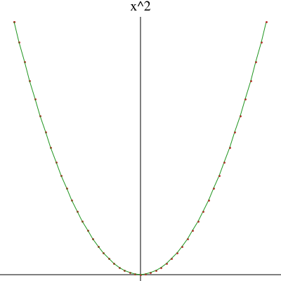
The left-hand side must be of type Symbol but the right-hand side can be a segment over any type.
sb := y = 1/2..3/2
SegmentBinding(Fraction(Integer)) The left- and right-hand sides can be obtained using the variable and segment operations.
variable(sb)
segment(sb)
For more information on related topics, see ‘Segment’ on page 1263 and ‘UniversalSegment’ on page 1365. Issue the system command )show SegmentBinding to display the full list of operations defined by SegmentBinding.
The Set domain allows one to represent explicit finite sets of values. These are similar to lists, but duplicate elements are not allowed. Sets can be created by giving a fixed set of values …
s := set [x^2-1, y^2-1, z^2-1]
Set(Polynomial(Integer)) or by using a collect form, just as for lists. In either case, the set is formed from a finite collection of values.
t := set [x^i - i+1 for i in 2..10 | prime? i]
The basic operations on sets are intersect, union, difference, and symmetricDifference.
i := intersect(s,t)
u := union(s,t)
Set(Polynomial(Integer)) The set difference(s,t) contains those members of s which are not in t.
difference(s,t)
Set(Polynomial(Integer)) The set symmetricDifference(s,t) contains those elements which are in s or t but not in
both.
symmetricDifference(s,t)
Set membership is tested using the member? operation.
member?(y, s)
member?((y+1)*(y-1), s)
Boolean The subset? function determines whether one set is a subset of another.
subset?(i, s)
subset?(u, s)
When the base type is finite, the absolute complement of a set is defined. This finds the set of all
multiplicative generators of PrimeField 11—the integers mod 11.
gs := set [g for i in 1..11 | primitive?(g := i::PF 11)]
Set(PrimeField(11)) The following values are not generators.
complement gs
Often the members of a set are computed individually; in addition, values can be inserted or removed from a set over the course of a computation. There are two ways to do this:
a := set [i^2 for i in 1..5]
Set(PositiveInteger) One is to view a set as a data structure and to apply updating operations.
insert!(32, a)
remove!(25, a)
a
Set(PositiveInteger) The other way is to view a set as a mathematical entity and to create new sets from old.
b := b0 := set [i^2 for i in 1..5]
b := union(b, {32})
b := difference(b, {25})
b0
For more information about lists, see ‘List’ on page 1074. Issue the system command )show Set to display the full list of operations defined by Set.
The SingleInteger domain is intended to provide support in FriCAS for machine integer arithmetic. It is generally much faster than (bignum) Integer arithmetic but suffers from a limited range of values. Since FriCAS can be implemented on top of various dialects of Lisp, the actual representation of small integers may not correspond exactly to the host machine’s integer representation.
The underlying Lisp primitives treat machine-word sized computations specially.
You can discover the minimum and maximum values in your implementation by using min and max.
min()$SingleInteger
max()$SingleInteger
SingleInteger To avoid confusion with Integer, which is the default type for integers, you usually need to work with declared variables (Section 2.3 on page 146) …
a := 1234 :: SingleInteger
SingleInteger or use package calling (Section 2.9 on page 179).
b := 124$SingleInteger
SingleInteger You can add, multiply and subtract SingleInteger objects, and ask for the greatest common divisor (gcd).
gcd(a,b)
SingleInteger The least common multiple (lcm) is also available.
lcm(a,b)
Operations mulmod, addmod, submod, and invmod are similar—they provide arithmetic modulo a given small
integer. Here is 5 * 6 mod 13.
mulmod(5,6,13)$SingleInteger
SingleInteger To reduce a small integer modulo a prime, use positiveRemainder.
positiveRemainder(37,13)$SingleInteger
SingleInteger Operations And, Or, xor, and Not provide bit level operations on small integers.
And(3,4)$SingleInteger
SingleInteger Use shift(int,numToShift) to shift bits, where i is shifted left if numToShift is positive, right if
negative.
shift(1,4)$SingleInteger
shift(31,-1)$SingleInteger
Many other operations are available for small integers, including many of those provided for Integer. To see the other operations, use the Browse HyperDoc facility (Section 14 on page 1513). Issue the system command )show SingleInteger to display the full list of operations defined by SingleInteger..
The SparseTable domain provides a general purpose table type with default entries. Here we create a table
to save strings under integer keys. The value "Try again!" is returned if no other value has been stored for a
key.
t: SparseTable(Integer, String, "Try again!") := table()
SparseTable(Integer, String, "Try again!") Entries can be stored in the table.
t.3 := "Number three"
t.4 := "Number four"
String These values can be retrieved as usual, but if a lookup fails the default entry will be returned.
t.3
t.2
String To see which values are explicitly stored, the keys and entries functions can be used.
keys t
entries t
List(String) If a specific table representation is required, the GeneralSparseTable constructor should be used. The domain SparseTable(K, E, dflt) is equivalent to GeneralSparseTable(K,E, Table(K,E), dflt). For more information, see ‘Table’ on page 1330 and ‘GeneralSparseTable’ on page 937. Issue the system command )show SparseTable to display the full list of operations defined by SparseTable.
The SquareFreeRegularTriangularSet domain constructor implements square-free regular triangular sets. See the RegularTriangularSet domain constructor for general regular triangular sets. Let T be a regular triangular set consisting of polynomials t1, ..., tm ordered by increasing main variables. The regular triangular set T is square-free if T is empty or if t1, ..., tm-1 is square-free and if the polynomial tm is square-free as a univariate polynomial with coefficients in the tower of simple extensions associated with t1, ..., tm-1.
The main interest of square-free regular triangular sets is that their associated towers of simple extensions are product of fields. Consequently, the saturated ideal of a square-free regular triangular set is radical. This property simplifies some of the operations related to regular triangular sets. However, building square-free regular triangular sets is generally more expensive than building general regular triangular sets.
Like the RegularTriangularSet domain constructor, the SquareFreeRegularTriangularSet domain constructor also implements a method for solving polynomial systems by means of regular triangular sets. This is in fact the same method with some adaptations to take into account the fact that the computed regular chains are square-free. Note that it is also possible to pass from a decomposition into general regular triangular sets to a decomposition into square-free regular triangular sets. This conversion is used internally by the LazardSetSolvingPackage package constructor.
N.B. When solving polynomial systems with the SquareFreeRegularTriangularSet domain constructor or the LazardSetSolvingPackage package constructor, decompositions have no redundant components. See also LexTriangularPackage and ZeroDimensionalSolvePackage for the case of algebraic systems with a finite number of (complex) solutions.
We shall explain now how to use the constructor SquareFreeRegularTriangularSet.
This constructor takes four arguments. The first one, R, is the coefficient ring of the polynomials; it must belong to the category GcdDomain. The second one, E, is the exponent monoid of the polynomials; it must belong to the category OrderedAbelianMonoidSup. The third one, V, is the ordered set of variables; it must belong to the category OrderedSet. The last one is the polynomial ring; it must belong to the category RecursivePolynomialCategory(R,E,V). The abbreviation for SquareFreeRegularTriangularSet is SREGSET.
Note that the way of understanding triangular decompositions is detailed in the example of the RegularTriangularSet constructor.
Let us illustrate the use of this constructor with one example (Donati-Traverso). Define the coefficient ring.
R := Integer
Type Define the list of variables,
ls : List Symbol := [x,y,z,t]
List(Symbol) and make it an ordered set;
V := OVAR(ls)
Type then define the exponent monoid.
E := IndexedExponents V
Type Define the polynomial ring.
P := NSMP(R, V)
Type Let the variables be polynomial.
x: P := ’x
NewSparseMultivariatePolynomial(Integer, OrderedVariableList([x, y, z, t]))
y: P := ’y
NewSparseMultivariatePolynomial(Integer, OrderedVariableList([x, y, z, t]))
z: P := ’z
NewSparseMultivariatePolynomial(Integer, OrderedVariableList([x, y, z, t]))
t: P := ’t
NewSparseMultivariatePolynomial(Integer, OrderedVariableList([x, y, z, t])) Now call the SquareFreeRegularTriangularSet domain constructor.
ST := SREGSET(R,E,V,P)
Type Define a polynomial system.
p1 := x ^ 31 - x ^ 6 - x - y
NewSparseMultivariatePolynomial(Integer, OrderedVariableList([x, y, z, t]))
p2 := x ^ 8 - z
NewSparseMultivariatePolynomial(Integer, OrderedVariableList([x, y, z, t]))
p3 := x ^ 10 - t
NewSparseMultivariatePolynomial(Integer, OrderedVariableList([x, y, z, t]))
lp := [p1, p2, p3]
List(NewSparseMultivariatePolynomial(Integer, OrderedVariableList([x, y, z, t])))
First of all, let us solve this system in the sense of Kalkbrener.
zeroSetSplit(lp)$ST
List(SquareFreeRegularTriangularSet(Integer, IndexedExponents(OrderedVariableList([x, y, z, t])), OrderedVariableList([x, y, z, t]), NewSparseMultivariatePolynomial(Integer, OrderedVariableList([x, y, z, t])))) And now in the sense of Lazard (or Wu and other authors).
zeroSetSplit(lp,false)$ST
Now to see the difference with the RegularTriangularSet domain constructor, we define:
T := REGSET(R,E,V,P)
Type and compute:
lts := zeroSetSplit(lp,false)$T
List(RegularTriangularSet(Integer, IndexedExponents(OrderedVariableList([x, y, z, t])), OrderedVariableList([x, y, z, t]), NewSparseMultivariatePolynomial(Integer, OrderedVariableList([x, y, z, t])))) If you look at the second set in both decompositions in the sense of Lazard, you will see that the polynomial with main variable y is not the same.
Let us understand what has happened. We define:
ts := lts.2
pol := select(ts,’y)$T
Union(NewSparseMultivariatePolynomial(Integer, OrderedVariableList([x, y, z, t])), ...)
tower := collectUnder(ts,’y)$T
pack := RegularTriangularSetGcdPackage(R,E,V,P,T)
Type Then we compute:
toseSquareFreePart(pol,tower)$pack
The top level matrix type in FriCAS is Matrix (see ‘Matrix’ on page 1113), which provides basic arithmetic and linear algebra functions. However, since the matrices can be of any size, it is not true that any pair can be added or multiplied. Thus Matrix has little algebraic structure.
Sometimes you want to use matrices as coefficients for polynomials or in other algebraic contexts. In this case,
SquareMatrix should be used. The domain SquareMatrix(n,R) gives the ring of n by n square matrices
over R.
Since SquareMatrix is not normally exposed at the top level, you must expose it before it can be used.
)set expose add constructor SquareMatrix
SquareMatrix is now explicitly exposed in frame initial
Once SQMATRIX has been exposed, values can be created using the squareMatrix function.
m := squareMatrix [[1,-%i],[%i,4]]
SquareMatrix(2, Complex(Integer)) The usual arithmetic operations are available.
m*m - m
SquareMatrix(2, Complex(Integer)) Square matrices can be used where ring elements are required. For example, here is a matrix with matrix entries.
mm := squareMatrix [[m, 1], [1-m, m^2]]
SquareMatrix(2, SquareMatrix(2, Complex(Integer))) Or you can construct a polynomial with square matrix coefficients.
p := (x + m)^2
Polynomial(SquareMatrix(2, Complex(Integer))) This value can be converted to a square matrix with polynomial coefficients.
p::SquareMatrix(2, ?)
SquareMatrix(2, Polynomial(Complex(Integer)))
For more information on related topics, see Section 2.2.4 on page 144, Section 2.11 on page 188, and ‘Matrix’ on page 1113. Issue the system command )show SquareMatrix to display the full list of operations defined by SquareMatrix.
A Stream object is represented as a list whose last element contains the wherewithal to create
the next element, should it ever be required. Let ints be the infinite stream of non-negative
integers.
ints := [i for i in 0..]
Stream(NonNegativeInteger) By default, ten stream elements are calculated. This number may be changed to something else by the system command )set streams calculate. For the display purposes of this book, we have chosen a smaller value. More generally, you can construct a stream by specifying its initial value and a function which, when given an element, creates the next element.
f : List INT -> List INT
f x == [x.1 + x.2, x.1]
fibs := [i.2 for i in [stream(f, [1, 1])]]
Compiling function f with type List(Integer) -> List(Integer)
Stream(Integer) You can create the stream of odd non-negative integers by either filtering them from the integers, or by evaluating an expression for each integer.
[i for i in ints | odd? i]
odds := [2*i+1 for i in ints]
Stream(NonNegativeInteger) You can accumulate the initial segments of a stream using the scan operation.
scan(0,+,odds)
Stream(NonNegativeInteger) The corresponding elements of two or more streams can be combined in this way.
[i*j for i in ints for j in odds]
map(*,ints,odds)
Stream(NonNegativeInteger) Many operations similar to those applicable to lists are available for streams.
first ints
rest ints
fibs 20
PositiveInteger The packages StreamFunctions1, StreamFunctions2 and StreamFunctions3 export some useful stream manipulation operations. For more information, see Section 5.5 on page 283, Section 8.9 on page 549, ‘ContinuedFraction’ on page 780, and ‘List’ on page 1074. Issue the system command )show Stream to display the full list of operations defined by Stream.
The type String provides character strings. Character strings provide all the operations for a one-dimensional array of characters, plus additional operations for manipulating text. For more information on related topics, see ‘Character’ on page 745 and ‘CharacterClass’ on page 751. You can also issue the system command )show String to display the full list of operations defined by String.
String values can be created using double quotes.
hello := "Hello, I’m FriCAS!"
String Note, however, that double quotes and underscores must be preceded by an extra underscore.
said := "Jane said, _"Look!_""
saw := "She saw exactly one underscore: __."
String It is also possible to use new to create a string of any size filled with a given character. Since there are many new functions it is necessary to indicate the desired type.
gasp: String := new(32, char "x")
String The length of a string is given by #.
#gasp
PositiveInteger Indexing operations allow characters to be extracted or replaced in strings. For any string s,
indices lie in the range 1..#s.
hello.2
Character Indexing is really just the application of a string to a subscript, so any application syntax works.
hello 2
hello(2)
Character If it is important not to modify a given string, it should be copied before any updating operations are used.
hullo := copy hello
hullo.2 := char "u"; [hello, hullo]
Operations are provided to split and join strings. The concat operation allows several strings to be joined together.
saidsaw := concat ["alpha","---”,”omega”]
String There is a version of concat that works with two strings.
concat("hello ","goodbye")
String Juxtaposition can also be used to concatenate strings.
"This " "is " "several " "strings " "concatenated."
String Substrings are obtained by giving an index range.
hello(1..5)
hello(8..)
String A string can be split into several substrings by giving a separation character or character class.
split(hello, char " ")
other := complement alphanumeric();
split(saidsaw, other)
List(String) Unwanted characters can be trimmed from the beginning or end of a string using the operations trim, leftTrim and rightTrim.
trim ("## ++ relax ++ ##", char "#")
String Each of these functions takes a string and a second argument to specify the characters to be discarded.
trim ("## ++ relax ++ ##", other)
String The second argument can be given either as a single character or as a character class.
leftTrim ("## ++ relax ++ ##", other)
rightTrim("## ++ relax ++ ##", other)
Strings can be changed to upper case or lower case using the operations upperCase, upperCase!, lowerCase and lowerCase!.
upperCase hello
String The versions with the exclamation mark change the original string, while the others produce a copy.
lowerCase hello
Some basic string matching is provided. The function prefix? tests whether one string is an initial prefix of another.
prefix?("He", "Hello")
prefix?("Her", "Hello")
Boolean A similar function, suffix?, tests for suffixes.
suffix?("", "Hello")
suffix?("LO", "Hello")
Boolean The function substring? tests for a substring given a starting position.
substring?("ll", "Hello", 3)
substring?("ll", "Hello", 4)
A number of position functions locate things in strings. If the first argument to position is a string,
then position(s,t,i) finds the location of s as a substring of t starting the search at position
i.
n := position("nd", "underground", 1)
n := position("nd", "underground", n+1)
PositiveInteger If s is not found, then 0 is returned (minIndex(s)-1 in IndexedString).
n := position("nd", "underground", n+1)
NonNegativeInteger To search for a specific character or a member of a character class, a different first argument is used.
position(char "d", "underground", 1)
position(hexDigit(), "underground", 1)
This domain provides a table type in which the keys are known to be strings, so special techniques can be used. Other than performance, the type StringTable(S) should behave exactly the same way as Table(String,S). See ‘Table’ on page 1330 for general information about tables. Issue the system command )show StringTable to display the full list of operations defined by StringTable.
This creates a new table whose keys are strings.
t: StringTable(Integer) := table()
StringTable(Integer) The value associated with each string key is the number of characters in the string.
for s in split("My name is Ian Watt.",char " ") repeat t.s := #s
for key in keys t repeat output [key, t.key]
["Watt.", 5]
["Ian", 3]
["is", 2]
["name", 4]
["My", 2]
Symbols are one of the basic types manipulated by FriCAS. The Symbol domain provides ways to create symbols of many varieties. Issue the system command )show Symbol to display the full list of operations defined by Symbol.
The simplest way to create a symbol is to “single quote” an identifier.
X: Symbol := ’x
Symbol This gives the symbol even if x has been assigned a value. If x has not been assigned a value, then
it is possible to omit the quote.
XX: Symbol := x
Symbol Declarations must be used when working with symbols, because otherwise the interpreter tries to place values in a more specialized type Variable.
A := ’a
B := b
Variable(b) The normal way of entering polynomials uses this fact.
x^2 + 1
Another convenient way to create symbols is to convert a string. This is useful when the name is to be constructed by a program.
"Hello"::Symbol
Symbol Sometimes it is necessary to generate new unique symbols, for example, to name constants of
integration. The expression new() generates a symbol starting with %.
new()$Symbol
Symbol Successive calls to new produce different symbols.
new()$Symbol
Symbol The expression new("s") produces a symbol starting with %s.
new("xyz")$Symbol
A symbol can be adorned in various ways. The most basic thing is applying a symbol to a list of subscripts.
X[i,j]
Somewhat less pretty is to attach subscripts, superscripts or arguments.
U := subscript(u, [1,2,1,2])
V := superscript(v, [n])
P := argscript(p, [t])
It is possible to test whether a symbol has scripts using the scripted? test.
scripted? U
scripted? X
Boolean If a symbol is not scripted, then it may be converted to a string.
string X
String The basic parts can always be extracted using the name and scripts operations.
name U
scripts U
name X
scripts X
The most general form is obtained using the script operation. This operation takes an argument which is a list containing, in this order, lists of subscripts, superscripts, presuperscripts, presubscripts and arguments to a symbol.
M := script(Mammoth, [[i,j],[k,l],[0,1],[2],[u,v,w]])
scripts M
Record(sub: List(OutputForm), sup: List(OutputForm), presup: List(OutputForm), presub: List(OutputForm), args: List(OutputForm)) If trailing lists of scripts are omitted, they are assumed to be empty.
N := script(Nut, [[i,j],[k,l],[0,1]])
scripts N
The Table constructor provides a general structure for associative storage. This type provides hash tables in which data objects can be saved according to keys of any type. For a given table, specific types must be chosen for the keys and entries.
In this example the keys to the table are polynomials with integer coefficients. The entries in the table are strings.
t: Table(Polynomial Integer, String) := table()
Table(Polynomial(Integer), String) To save an entry in the table, the setelt! operation is used. This can be called directly, giving the table a key and an entry.
setelt!(t, x^2 - 1, "Easy to factor")
String Alternatively, you can use assignment syntax.
t(x^3 + 1) := "Harder to factor"
t(x) := "The easiest to factor"
String Entries are retrieved from the table by calling the elt operation.
elt(t, x)
String This operation is called when a table is “applied” to a key using this or the following syntax.
t.x
t x
String Parentheses are used only for grouping. They are needed if the key is an infixed expression.
t.(x^2 - 1)
String Note that the elt operation is used only when the key is known to be in the table—otherwise an error is generated.
t (x^3 + 1)
You can get a list of all the keys to a table using the keys operation.
keys t
List(Polynomial(Integer)) If you wish to test whether a key is in a table, the search operation is used. This operation
returns either an entry or "failed".
search(x, t)
search(x^2, t)
Union("failed", ...) The return type is a union so the success of the search can be tested using case.
search(x^2, t) case "failed"
Boolean The remove! operation is used to delete values from a table.
remove!(x^2-1, t)
Union(String, ...) If an entry exists under the key, then it is returned. Otherwise remove! returns
"failed".
remove!(x-1, t)
The number of key-entry pairs can be found using the # operation.
#t
PositiveInteger Just as keys returns a list of keys to the table, a list of all the entries can be obtained using the members operation.
members t
List(String) A number of useful operations take functions and map them on to the table to compute the
result. Here we count the entries which have "Hard" as a prefix.
count(s: String +-> prefix?("Hard", s), t)
Other table types are provided to support various needs.
Issue the system command )show Table to display the full list of operations defined by Table.
The domain TextFile allows FriCAS to read and write character data and exchange text with other programs. This type behaves in FriCAS much like a File of strings, with additional operations to cause new lines. We give an example of how to produce an upper case copy of a file. This is the file from which we read the text.
f1: TextFile := open("/etc/group", "input")
TextFile This is the file to which we write the text.
f2: TextFile := open("/tmp/MOTD", "output")
TextFile Entire lines are handled using the readLine! and writeLine! operations.
l := readLine! f1
writeLine!(f2, upperCase l)
String Use the endOfFile? operation to check if you have reached the end of the file.
while not endOfFile? f1 repeat s := readLine! f1 writeLine!(f2, upperCase s)
The file f1 is exhausted and should be closed.
close! f1
It is sometimes useful to write lines a bit at a time. The write! operation allows this.
write!(f2, "-The-")
write!(f2, "-End-")
String This ends the line. This is done in a machine-dependent manner.
writeLine! f2
close! f2
TextFile Finally, clean up.
)system rm /tmp/MOTD
For more information on related topics, see ‘File’ on page 876, ‘KeyedAccessFile’ on page 997, and ‘Library’ on page 1031. Issue the system command )show TextFile to display the full list of operations defined by TextFile.
The TwoDimensionalArray domain is used for storing data in a two-dimensional data structure indexed by
row and by column. Such an array is a homogeneous data structure in that all the entries of the array must
belong to the same FriCAS domain (although see Section 2.6 on page 166). Each array has a fixed number of
rows and columns specified by the user and arrays are not extensible. In FriCAS, the indexing of
two-dimensional arrays is one-based. This means that both the “first” row of an array and the “first” column
of an array are given the index 1. Thus, the entry in the upper left corner of an array is in position
(1,1).
The operation new creates an array with a specified number of rows and columns and fills the components of that array with a specified entry. The arguments of this operation specify the number of rows, the number of columns, and the entry. This creates a five-by-four array of integers, all of whose entries are zero.
arr : ARRAY2 INT := new(5,4,0)
TwoDimensionalArray(Integer) The entries of this array can be set to other integers using the operation setelt!.
Issue this to set the element in the upper left corner of this array to 17.
setelt!(arr, 1, 1, 17)
PositiveInteger Now the first element of the array is 17.
arr
TwoDimensionalArray(Integer) Likewise, elements of an array are extracted using the operation elt.
elt(arr,1,1)
PositiveInteger Another way to use these two operations is as follows. This sets the element in position (3,2) of
the array to 15.
arr(3,2) := 15
PositiveInteger This extracts the element in position (3,2) of the array.
arr(3,2)
PositiveInteger The operations elt and setelt! come equipped with an error check which verifies that the indices are
in the proper ranges. For example, the above array has five rows and four columns, so if you ask
for the entry in position (6,2) with arr(6,2) FriCAS displays an error message. If there is no
need for an error check, you can call the operations qelt and qsetelt! which provide the same
functionality but without the error check. Typically, these operations are called in well-tested
programs.
The operations row and column extract rows and columns, respectively, and return objects of OneDimensionalArray with the same underlying element type.
row(arr,1)
column(arr,1)
You can determine the dimensions of an array by calling the operations nrows and ncols, which return the number of rows and columns, respectively.
nrows(arr)
ncols(arr)
PositiveInteger To apply an operation to every element of an array, use map. This creates a new array. This expression negates every element.
map(-,arr)
TwoDimensionalArray(Integer) This creates an array where all the elements are doubled.
map((x +-> x + x),arr)
TwoDimensionalArray(Integer) To change the array destructively, use map! instead of map. If you need to make a copy of any array, use copy.
arrc := copy(arr)
map!(-,arrc)
arrc
arr
Use member? to see if a given element is in an array.
member?(17,arr)
member?(10317,arr)
Boolean To see how many times an element appears in an array, use count.
count(17,arr)
count(0,arr)
For more information about the operations available for TwoDimensionalArray, issue )show TwoDimensionalArray. For information on related topics, see ‘Matrix’ on page 1113 and ‘OneDimensionalArray’ on page 1147.
The domain constructor UnivariatePolynomial (abbreviated UP) creates domains of univariate
polynomials in a specified variable. For example, the domain UP(a1,POLY FRAC INT) provides
polynomials in the single variable a1 whose coefficients are general polynomials with rational number
coefficients.
UP(x,INT) is the domain of polynomials in the single variable x with integer coefficients.
(p,q) : UP(x,INT)
p := (3*x-1)^2 * (2*x + 8)
UnivariatePolynomial(x, Integer)
q := (1 - 6*x + 9*x^2)^2
UnivariatePolynomial(x, Integer) The usual arithmetic operations are available for univariate polynomials.
p^2 + p*q
UnivariatePolynomial(x, Integer) The operation leadingCoefficient extracts the coefficient of the term of highest degree.
leadingCoefficient p
PositiveInteger The operation degree returns the degree of the polynomial. Since the polynomial has only one variable, the variable is not supplied to operations like degree.
degree p
PositiveInteger The reductum of the polynomial, the polynomial obtained by subtracting the term of highest order, is returned by reductum.
reductum p
UnivariatePolynomial(x, Integer) The operation gcd computes the greatest common divisor of two polynomials.
gcd(p,q)
UnivariatePolynomial(x, Integer) The operation lcm computes the least common multiple.
lcm(p,q)
UnivariatePolynomial(x, Integer) The operation resultant computes the resultant of two univariate
polynomials. In the case of p and q, the resultant is 0 because they share a common root.
resultant(p,q)
NonNegativeInteger To compute the derivative of a univariate polynomial with respect to its variable, use D.
D p
UnivariatePolynomial(x, Integer) Univariate polynomials can also be used as if they were functions. To evaluate a univariate polynomial at some point, apply the polynomial to the point.
p(2)
PositiveInteger The same syntax is used for composing two univariate polynomials, i.e. substituting one
polynomial for the variable in another. This substitutes q for the variable in p.
p(q)
UnivariatePolynomial(x, Integer) This substitutes p for the variable in q.
q(p)
UnivariatePolynomial(x, Integer) To obtain a list of coefficients of the polynomial, use coefficients.
l := coefficients p
List(Integer) From this you can use gcd and reduce to compute the content of the polynomial.
reduce(gcd,l)
PositiveInteger Alternatively (and more easily), you can just call content.
content p
Note that the operation coefficients omits the zero coefficients from the list. Sometimes it is useful to convert a
univariate polynomial to a vector whose  position contains the degree
i-1 coefficient of the
polynomial.
ux := (x^4+2*x+3)::UP(x,INT)
UnivariatePolynomial(x, Integer) To get a complete vector of coefficients, use the operation vectorise, which takes a univariate polynomial and an integer denoting the length of the desired vector.
vectorise(ux,5)
It is common to want to do something to every term of a polynomial, creating a new polynomial in the process. This is a function for iterating across the terms of a polynomial, squaring each term.
squareTerms(p) == reduce(+,[t^2 for t in monomials p])
Recall what p looked like.
p
UnivariatePolynomial(x, Integer) We can demonstrate squareTerms on p.
squareTerms p
Compiling function squareTerms with type UnivariatePolynomial(x,Integer) -> UnivariatePolynomial(x,Integer)
UnivariatePolynomial(x, Integer)
When the coefficients of the univariate polynomial belong to a field,7 it is possible to compute quotients and remainders.
(r,s) : UP(a1,FRAC INT)
r := a1^2 - 2/3
UnivariatePolynomial(a1, Fraction(Integer))
s := a1 + 4
UnivariatePolynomial(a1, Fraction(Integer)) When the coefficients are rational numbers or rational expressions, the operation quo computes the quotient of two polynomials.
r quo s
UnivariatePolynomial(a1, Fraction(Integer)) The operation rem computes the remainder.
r rem s
UnivariatePolynomial(a1, Fraction(Integer)) The operation divide can be used to return a record of both components.
d := divide(r, s)
Record(quotient: UnivariatePolynomial(a1, Fraction(Integer)), remainder: UnivariatePolynomial(a1, Fraction(Integer))) Now we check the arithmetic!
r - (d.quotient * s + d.remainder)
UnivariatePolynomial(a1, Fraction(Integer)) It is also possible to integrate univariate polynomials when the coefficients belong to a field.
integrate r
UnivariatePolynomial(a1, Fraction(Integer))
integrate s
UnivariatePolynomial(a1, Fraction(Integer))
One application of univariate polynomials is to see expressions in terms of a specific variable. We start with
a polynomial in a1 whose coefficients are quotients of polynomials in b1 and b2.
t : UP(a1,FRAC POLY INT)
Since in this case we are not talking about using multivariate polynomials in only two variables, we use Polynomial. We also use Fraction because we want fractions.
t := a1^2 - a1/b2 + (b1^2-b1)/(b2+3)
UnivariatePolynomial(a1, Fraction(Polynomial(Integer))) We push all the variables into a single quotient of polynomials.
u : FRAC POLY INT := t
Fraction(Polynomial(Integer)) Alternatively, we can view this as a polynomial in the variable This is a mode-directed conversion: you indicate as much of the structure as you care about and let FriCAS decide on the full type and how to do the transformation.
u :: UP(b1,?)
UnivariatePolynomial(b1, Fraction(Polynomial(Integer)))
See Section 8.2 on page 498 for a discussion of the factorization facilities in FriCAS for univariate polynomials. For more information on related topics, see Section 1.9 on page 95, Section 2.7 on page 167, ‘Polynomial’ on page 1183, ‘MultivariatePolynomial’ on page 1135, and ‘DistributedMultivariatePolynomial’ on page 830. Issue the system command )show UnivariatePolynomial to display the full list of operations defined by UnivariatePolynomial.
The UniversalSegment domain generalizes Segment by allowing segments without a “high” end point.
pints := 1..
UniversalSegment(PositiveInteger)
nevens := (0..) by -2
UniversalSegment(NonNegativeInteger) Values of type Segment are automatically converted to type UniversalSegment when appropriate.
useg: UniversalSegment(Integer) := 3..10
UniversalSegment(Integer) The operation hasHi is used to test whether a segment has a high end
point.
hasHi pints
hasHi nevens
hasHi useg
Boolean All operations available on type Segment apply to UniversalSegment, with the proviso that expansions produce streams rather than lists. This is to accommodate infinite expansions.
expand pints
expand nevens
expand [1, 3, 10..15, 100..]
For more information on related topics, see ‘Segment’ on page 1263, ‘SegmentBinding’ on page 1268, ‘List’ on page 1074, and ‘Stream’ on page 1300. Issue the system command )show UniversalSegment to display the full list of operations defined by UniversalSegment.
The Vector domain is used for storing data in a one-dimensional indexed data structure. A vector is a homogeneous data structure in that all the components of the vector must belong to the same FriCAS domain. Each vector has a fixed length specified by the user; vectors are not extensible. This domain is similar to the OneDimensionalArray domain, except that when the components of a Vector belong to a Ring, arithmetic operations are provided. For more examples of operations that are defined for both Vector and OneDimensionalArray, see ‘OneDimensionalArray’ on page 1147.
As with the OneDimensionalArray domain, a Vector can be created by calling the operation new, its
components can be accessed by calling the operations elt and qelt, and its components can be reset by calling
the operations setelt! and qsetelt!. This creates a vector of integers of length 5 all of whose components are
12.
u : VECTOR INT := new(5,12)
Vector(Integer) This is how you create a vector from a list of its components.
v : VECTOR INT := vector([1,2,3,4,5])
Indexing for vectors begins at 1. The last element has index equal to the length of the vector, which is
computed by #.
#(v)
PositiveInteger This is the standard way to use elt to extract an element. Functionally, it is the same as if you had
typed elt(v,2).
v.2
PositiveInteger This is the standard way to use setelt! to change an element. It is the same as if you had typed
setelt!(v, 3, 99).
v.3 := 99
PositiveInteger Now look at v to see the change. You can use qelt and qsetelt! (instead of elt and setelt!,
respectively) but only when you know that the index is within the valid range.
v
When the components belong to a Ring, FriCAS provides arithmetic operations for Vector. These include left and right scalar multiplication.
5 * v
v * 7
w : VECTOR INT := vector([2,3,4,5,6])
Vector(Integer) Addition and subtraction are also available.
v + w
Vector(Integer) Of course, when adding or subtracting, the two vectors must have the same length or an error message is displayed.
v - w
For more information about other aggregate domains, see the following: ‘List’ on page 1074, ‘Matrix’ on page 1113, ‘OneDimensionalArray’ on page 1147, ‘Set’ on page 1271, ‘Table’ on page 1330, and ‘TwoDimensionalArray’ on page 1342. Issue the system command )show Vector to display the full list of operations defined by Vector.
When an expression is not in a value context, it is given type Void. For example, in the expression
r := (a; b; if c then d else e; f)
values are used only from the subexpressions c and f: all others are thrown away. The subexpressions a, b, d
and e are evaluated for side-effects only and have type Void. There is a unique value of type
Void.
You will most often see results of type Void when you declare a variable.
a : Integer
Usually no output is displayed for Void results. You can force the display of a rather ugly object by issuing )set message void on.
)set message void on
b : Fraction Integer
)set message void off
All values can be converted to type Void.
3::Void
Once a value has been converted to Void, it cannot be recovered.
% :: PositiveInteger
Cannot convert the value from type Void to PositiveInteger .
The WuWenTsunTriangularSet domain constructor implements the characteristic set method of Wu Wen Tsun. This algorithm computes a list of triangular sets from a list of polynomials such that the algebraic variety defined by the given list of polynomials decomposes into the union of the regular-zero sets of the computed triangular sets. The constructor takes four arguments. The first one, R, is the coefficient ring of the polynomials; it must belong to the category IntegralDomain. The second one, E, is the exponent monoid of the polynomials; it must belong to the category OrderedAbelianMonoidSup. The third one, V, is the ordered set of variables; it must belong to the category OrderedSet. The last one is the polynomial ring; it must belong to the category RecursivePolynomialCategory(R,E,V). The abbreviation for WuWenTsunTriangularSet is WUTSET.
Let us illustrate the facilities by an example.
Define the coefficient ring.
R := Integer
Type Define the list of variables,
ls : List Symbol := [x,y,z,t]
List(Symbol) and make it an ordered set;
V := OVAR(ls)
Type then define the exponent monoid.
E := IndexedExponents V
Type Define the polynomial ring.
P := NSMP(R, V)
Type Let the variables be polynomial.
x: P := ’x
NewSparseMultivariatePolynomial(Integer, OrderedVariableList([x, y, z, t]))
y: P := ’y
NewSparseMultivariatePolynomial(Integer, OrderedVariableList([x, y, z, t]))
z: P := ’z
NewSparseMultivariatePolynomial(Integer, OrderedVariableList([x, y, z, t]))
t: P := ’t
NewSparseMultivariatePolynomial(Integer, OrderedVariableList([x, y, z, t])) Now call the WuWenTsunTriangularSet domain constructor.
T := WUTSET(R,E,V,P)
Type Define a polynomial system.
p1 := x ^ 31 - x ^ 6 - x - y
NewSparseMultivariatePolynomial(Integer, OrderedVariableList([x, y, z, t]))
p2 := x ^ 8 - z
NewSparseMultivariatePolynomial(Integer, OrderedVariableList([x, y, z, t]))
p3 := x ^ 10 - t
NewSparseMultivariatePolynomial(Integer, OrderedVariableList([x, y, z, t]))
lp := [p1, p2, p3]
List(NewSparseMultivariatePolynomial(Integer, OrderedVariableList([x, y, z, t]))) Compute a characteristic set of the system.
characteristicSet(lp)$T
zeroSetSplit(lp)$T
The RegularTriangularSet and SquareFreeRegularTriangularSet domain constructors, and the LazardSetSolvingPackage, SquareFreeRegularTriangularSet and ZeroDimensionalSolvePackage package constructors also provide operations to compute triangular decompositions of algebraic varieties. These five constructor use a special kind of characteristic sets, called regular triangular sets. These special characteristic sets have better properties than the general ones. Regular triangular sets and their related concepts are presented in the paper ”On the Theories of Triangular sets” By P. Aubry, D. Lazard and M. Moreno Maza (to appear in the Journal of Symbolic Computation). The decomposition algorithm (due to the third author) available in the four above constructors provide generally better timings than the characteristic set method. In fact, the WUTSET constructor remains interesting for the purpose of manipulating characteristic sets whereas the other constructors are more convenient for solving polynomial systems.
Note that the way of understanding triangular decompositions is detailed in the example of the RegularTriangularSet constructor.
Initialisations
a:Symbol := ’a
b:Symbol := ’b
RN := Fraction(Integer)
word := FreeMonoid Symbol
lword := LyndonWord(Symbol)
base := PoincareBirkhoffWittLyndonBasis Symbol
dpoly := XDistributedPolynomial(Symbol, RN)
rpoly := XRecursivePolynomial(Symbol, RN)
lpoly := LiePolynomial(Symbol, RN)
poly := XPBWPolynomial(Symbol, RN)
liste : List lword := LyndonWordsList([a,b], 6)
Let’s make some polynomials
0$poly
XPBWPolynomial(Symbol, Fraction(Integer))
1$poly
XPBWPolynomial(Symbol, Fraction(Integer))
p : poly := a
XPBWPolynomial(Symbol, Fraction(Integer))
q : poly := b
XPBWPolynomial(Symbol, Fraction(Integer))
pq: poly := p*q
XPBWPolynomial(Symbol, Fraction(Integer)) Coerce to distributed polynomial
pq :: dpoly
XDistributedPolynomial(Symbol, Fraction(Integer))
Check some polynomial operations
mirror pq
XPBWPolynomial(Symbol, Fraction(Integer))
listOfTerms pq
List(Record(k: PoincareBirkhoffWittLyndonBasis(Symbol), c: Fraction(Integer)))
reductum pq
XPBWPolynomial(Symbol, Fraction(Integer))
leadingMonomial pq
XPBWPolynomial(Symbol, Fraction(Integer))
coefficients pq
leadingTerm pq
Record(k: PoincareBirkhoffWittLyndonBasis(Symbol), c: Fraction(Integer))
degree pq
pq4:=exp(pq,4)
XPBWPolynomial(Symbol, Fraction(Integer))
log(pq4,4) - pq
XPBWPolynomial(Symbol, Fraction(Integer))
Calculations with verification in XDistributedPolynomial.
lp1 :lpoly := LiePoly liste.10
LiePolynomial(Symbol, Fraction(Integer))
lp2 :lpoly := LiePoly liste.11
LiePolynomial(Symbol, Fraction(Integer))
lp :lpoly := [lp1, lp2]
LiePolynomial(Symbol, Fraction(Integer))
lpd1: dpoly := lp1
XDistributedPolynomial(Symbol, Fraction(Integer))
lpd2: dpoly := lp2
XDistributedPolynomial(Symbol, Fraction(Integer))
lpd : dpoly := lpd1 * lpd2 - lpd2 * lpd1
XDistributedPolynomial(Symbol, Fraction(Integer))
lp :: dpoly - lpd
XDistributedPolynomial(Symbol, Fraction(Integer))
Calculations with verification in XRecursivePolynomial.
p := 3 * lp
XPBWPolynomial(Symbol, Fraction(Integer))
q := lp1
XPBWPolynomial(Symbol, Fraction(Integer))
pq:= p * q
XPBWPolynomial(Symbol, Fraction(Integer))
pr:rpoly := p :: rpoly
XRecursivePolynomial(Symbol, Fraction(Integer))
qr:rpoly := q :: rpoly
XRecursivePolynomial(Symbol, Fraction(Integer))
pq :: rpoly - pr*qr
XRecursivePolynomial(Symbol, Fraction(Integer))
The XPolynomial domain constructor implements multivariate polynomials whose set of variables is Symbol. These variables do not commute. The only parameter of this constructor is the coefficient ring which may be non-commutative. However, coefficients and variables commute. The representation of the polynomials is recursive. The abbreviation for XPolynomial is XPOLY.
Other constructors like XPolynomialRing, XRecursivePolynomial, XDistributedPolynomial, LiePolynomial and XPBWPolynomial implement multivariate polynomials in non-commutative variables.
We illustrate now some of the facilities of the XPOLY domain constructor.
Define a polynomial ring over the integers.
poly := XPolynomial(Integer)
Define a first polynomial,
pr: poly := 2*x + 3*y-5
and a second one.
pr2: poly := pr*pr
Rewrite pr in a distributive way,
pd := expand pr
XDistributedPolynomial(Symbol, Integer)
compute its square,
pd2 := pd*pd
XDistributedPolynomial(Symbol, Integer)
and checks that:
expand(pr2) - pd2
XDistributedPolynomial(Symbol, Integer)
We define:
qr := pr^3
and:
qd := pd^3
XDistributedPolynomial(Symbol, Integer)
We truncate qd at degree 3:
trunc(qd,2)
XDistributedPolynomial(Symbol, Integer)
The same for qr:
trunc(qr,2)
We define:
Word := FreeMonoid Symbol
and:
w: Word := x*y^2
The we can compute the right-quotient of qr by r:
rquo(qr,w)
and the shuffle-product of pr by r:
sh(pr,w::poly)
The XPolynomialRing domain constructor implements generalized polynomials with coefficients from an arbitrary Ring (not necessarily commutative) and whose exponents are words from an arbitrary OrderedMonoid (not necessarily commutative too). Thus these polynomials are (finite) linear combinations of words.
This constructor takes two arguments. The first one is a Ring and the second is an OrderedMonoid. The abbreviation for XPolynomialRing is XPR.
Other constructors like XPolynomial, XRecursivePolynomial, XDistributedPolynomial, LiePolynomial and XPBWPolynomial implement multivariate polynomials in non-commutative variables.
We illustrate now some of the facilities of the XPR domain constructor.
Define the free ordered monoid generated by the symbols.
Word := FreeMonoid(Symbol)
Define the linear combinations of these words with integer coefficients.
poly:= XPR(Integer,Word)
Then we define a first element from poly.
p:poly := 2 * x - 3 * y + 1
XPolynomialRing(Integer, FreeMonoid(Symbol))
And a second one.
q:poly := 2 * x + 1
XPolynomialRing(Integer, FreeMonoid(Symbol))
We compute their sum,
p + q
XPolynomialRing(Integer, FreeMonoid(Symbol))
their product,
p * q
XPolynomialRing(Integer, FreeMonoid(Symbol))
and see that variables do not commute.
(p +q)^2 -p^2 -q^2 - 2*p*q
XPolynomialRing(Integer, FreeMonoid(Symbol))
Now we define a ring of square matrices,
M := SquareMatrix(2,Fraction Integer)
and the linear combinations of words with these matrices as coefficients.
poly1:= XPR(M,Word)
Define a first matrix,
m1:M := matrix [[i*j^2 for i in 1..2] for j in 1..2]
SquareMatrix(2, Fraction(Integer))
a second one,
m2:M := m1 - 5/4
SquareMatrix(2, Fraction(Integer))
and a third one.
m3: M := m2^2
SquareMatrix(2, Fraction(Integer))
Define a polynomial,
pm:poly1 := m1*x + m2*y + m3*z - 2/3
XPolynomialRing(SquareMatrix(2, Fraction(Integer)), FreeMonoid(Symbol))
a second one,
qm:poly1 := pm - m1*x
XPolynomialRing(SquareMatrix(2, Fraction(Integer)), FreeMonoid(Symbol))
and the following power.
qm^3
XPolynomialRing(SquareMatrix(2, Fraction(Integer)), FreeMonoid(Symbol))
The ZeroDimensionalSolvePackage package constructor provides operations for computing symbolically the complex or real roots of zero-dimensional algebraic systems.
The package provides no multiplicity information (i.e. some returned roots may be double or higher) but only distinct roots are returned.
Complex roots are given by means of univariate representations of irreducible regular chains. These representations are computed by the univariateSolve operation (by calling the InternalRationalUnivariateRepresentationPackage package constructor which does the job).
Real roots are given by means of tuples of coordinates lying in the RealClosure of the coefficient ring. They are computed by the realSolve and positiveSolve operations. The former computes all the solutions of the input system with real coordinates whereas the later concentrate on the solutions with (strictly) positive coordinates. In both cases, the computations are performed by the RealClosure constructor.
Both computations of complex roots and real roots rely on triangular decompositions. These decompositions can be computed in two different ways. First, by a applying the zeroSetSplit operation from the REGSET domain constructor. In that case, no Groebner bases are computed. This strategy is used by default. Secondly, by applying the zeroSetSplit from LEXTRIPK. To use this later strategy with the operations univariateSolve, realSolve and positiveSolve one just needs to use an extra boolean argument.
Note that the way of understanding triangular decompositions is detailed in the example of the RegularTriangularSet constructor.
The ZeroDimensionalSolvePackage constructor takes three arguments. The first one R is the coefficient ring; it must belong to the categories OrderedRing, EuclideanDomain, CharacteristicZero and RealConstant. This means essentially that R is Integer or Fraction(Integer). The second argument ls is the list of variables involved in the systems to solve. The third one MUST BE concat(ls,s) where s is an additional symbol used for the univariate representations. The abbreviation for ZeroDimensionalSolvePackage is ZDSOLVE.
We illustrate now how to use the constructor ZDSOLVE by two examples: the Arnborg and Lazard system and the L-3 system (Aubry and Moreno Maza). Note that the use of this package is also demonstrated in the example of the LexTriangularPackage constructor.
Define the coefficient ring.
R := Integer
Define the lists of variables:
ls : List Symbol := [x,y,z,t]
and:
ls2 : List Symbol := [x,y,z,t,new()$Symbol]
Call the package:
pack := ZDSOLVE(R,ls,ls2)
Define a polynomial system (Arnborg-Lazard)
p1 := x^2*y*z + x*y^2*z + x*y*z^2 + x*y*z + x*y + x*z + y*z
p2 := x^2*y^2*z + x*y^2*z^2 + x^2*y*z + x*y*z + y*z + x + z
p3 := x^2*y^2*z^2 + x^2*y^2*z + x*y^2*z + x*y*z + x*z + z + 1
lp := [p1, p2, p3]
List(Polynomial(Integer)) Note that these polynomials do not involve the variable t; we will use it in the second example.
First compute a decomposition into regular chains (i.e. regular triangular sets).
triangSolve(lp)$pack
List(RegularChain(Integer, [x, y, z, t]))
We can see easily from this decomposition (consisting of a single regular chain) that the input system has 20 complex roots.
Then we compute a univariate representation of this regular chain.
univariateSolve(lp)$pack
We see that the zeros of our regular chain are split into three components. This is due to the use of univariate polynomial factorization.
Each of these components consist of two parts. The first one is an irreducible univariate polynomial p(?) which defines a simple algebraic extension of the field of fractions of R. The second one consists of multivariate polynomials pol1(x,%A), pol2(y,%A) and pol3(z,%A). Each of these polynomials involve two variables: one is an indeterminate x, y or z of the input system lp and the other is %A which represents any root of p(?). Recall that this %A is the last element of the third parameter of ZDSOLVE. Thus any complex root ? of p(?) leads to a solution of the input system lp by replacing %A by this ? in pol1(x,%A), pol2(y,%A) and pol3(z,%A). Note that the polynomials pol1(x,%A), pol2(y,%A) and pol3(z,%A) have degree one w.r.t. x, y or z respectively. This is always the case for all univariate representations. Hence the operation univariateSolve replaces a system of multivariate polynomials by a list of univariate polynomials, what justifies its name. Another example of univariate representations illustrates the LexTriangularPackage package constructor.
We now compute the solutions with real coordinates:
lr := realSolve(lp)$pack;
List(List(RealClosure(Fraction(Integer))))
The number of real solutions for the input system is:
# lr
Each of these real solutions is given by a list of elements in RealClosure(R). In these 8 lists, the first
element is a value of z, the second of y and the last of x. This is logical since by setting the list of variables of
the package to [x,y,z,t] we mean that the elimination ordering on the variables is  . Note that
each system treated by the ZDSOLVE package constructor needs only to be zero-dimensional w.r.t. the
variables involved in the system it-self and not necessarily w.r.t. all the variables used to define the
package.
We can approximate these real numbers as follows. This computation takes between 30 sec. and 5 min, depending on your machine.
[[approximate(r,1/1000000) for r in point] for point in lr];
We can also concentrate on the solutions with real (strictly) positive coordinates:
lpr := positiveSolve(lp)$pack
List(List(RealClosure(Fraction(Integer))))
Thus we have checked that the input system has no solution with strictly positive coordinates.
Let us define another polynomial system (L-3).
f0 := x^3 + y + z + t- 1
f1 := x + y^3 + z + t -1
f2 := x + y + z^3 + t-1
f3 := x + y + z + t^3 -1
lf := [f0, f1, f2, f3]
First compute a decomposition into regular chains (i.e. regular triangular sets).
lts := triangSolve(lf)$pack
List(RegularChain(Integer, [x, y, z, t]))
Then we compute a univariate representation.
univariateSolve(lf)$pack
Note that this computation is made from the input system lf. However it is possible to reuse a pre-computed regular chain as follows:
ts := lts.1
RegularChain(Integer, [x, y, z, t])
univariateSolve(ts)$pack
realSolve(ts)$pack
List(List(RealClosure(Fraction(Integer))))
We compute now the full set of points with real coordinates:
lr2 := realSolve(lf)$pack;
List(List(RealClosure(Fraction(Integer))))
The number of real solutions for the input system is:
#lr2
PositiveInteger Another example of computation of real solutions illustrates the LexTriangularPackage package constructor.
We concentrate now on the solutions with real (strictly) positive coordinates:
lpr2 := positiveSolve(lf)$pack
List(List(RealClosure(Fraction(Integer))))
Finally, we approximate the coordinates of this point with 20 exact digits:
[approximate(r,1/10^21)::Float for r in lpr2.1]
Programming in the interpreter is easy. So is the use of FriCAS’s graphics facility. Both are rather flexible and allow you to use them for many interesting applications. However, both require learning some basic ideas and skills.
All graphics examples in the FriCAS Images section are either produced directly by interactive commands or by interpreter programs. Four of these programs are introduced here. By the end of this chapter you will know enough about graphics and programming in the interpreter to not only understand all these examples, but to tackle interesting and difficult problems on your own. Appendix A.27 lists all the remaining commands and programs used to create these images.
We begin our discussion of interactive graphics with the creation of a useful facility: plotting ribbons of
two-dimensional graphs in three-dimensional space. Suppose you want to draw the two-dimensional graphs of
 functions
 all over some fixed range of
 . One approach is to create a two-dimensional
graph for each one, then superpose one on top of the other. What you will more than likely get
is a jumbled mess. Even if you make each function a different color, the result is likely to be
confusing.
A better approach is to display each of the  in three dimensions as a “ribbon” of some appropriate
width along the
 -direction, laying down each ribbon next to the previous one. A ribbon is simply a function
of
 and
 depending only on

We illustrate this for  defined as simple powers of
 for
 ranging between
 and
 .
Draw the ribbon for  .
draw(x^2,x=-1..1,y=0..1)
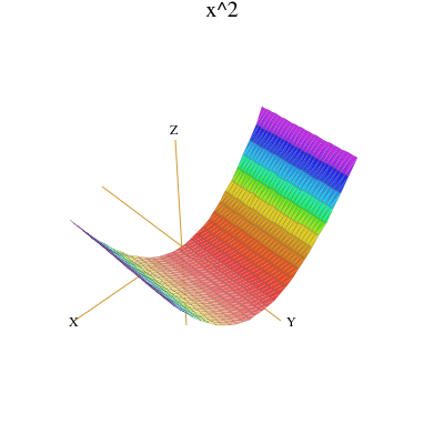
Now that was easy! What you get is a “wire-mesh” rendition of the ribbon. That’s fine for now. Notice that
the mesh-size is small in both the  and the
 directions. FriCAS normally computes points in both these
directions. This is unnecessary. One step is all we need in the
 -direction. To have FriCAS economize on
y-points, we re-draw the ribbon with option var2Steps == 1.
Re-draw the ribbon, but with option var2Steps == 1 so that only 1 step is computed in the  direction.
vp := draw(x^2,x=-1..1,y=0..1,var2Steps==1)
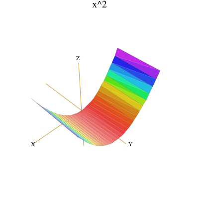
The operation has created a viewport, that is, a graphics window on your screen. We assigned the viewport to
vp and now we manipulate its contents.
Graphs are objects, like numbers and algebraic expressions. You may want to do some experimenting with graphs. For example, say
showRegion(vp, "on")
to put a bounding box around the ribbon. Try it! Issue rotate(vp, -45, 90) to rotate the figure  longitudinal degrees and
 latitudinal degrees.
Here is a different rotation. This turns the graph so you can view it along the  -axis.
rotate(vp, 0, -90)
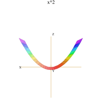
There are many other things you can do. In fact, most everything you can do interactively using the three-dimensional control panel (such as translating, zooming, resizing, coloring, perspective and lighting selections) can also be done directly by operations (see Chapter 7 for more details).
When you are done experimenting, say reset(vp) to restore the picture to its original position and
settings.
Let’s add another ribbon to our picture—one for  . Since
 ranges from
 to
 for the first ribbon, now
let
 range from
 to
 This puts the second ribbon next to the first one.
How do you add a second ribbon to the viewport? One method is to extract the “space” component from the
viewport using the operation subspace. You can think of the space component as the object inside the window
(here, the ribbon). Let’s call it sp. To add the second ribbon, you draw the second ribbon using the option
space == sp.
Extract the space component of vp.
sp := subspace(vp)
Add the ribbon for  alongside that for
 .
vp := draw(x^3,x=-1..1,y=1..2,var2Steps==1, space==sp)
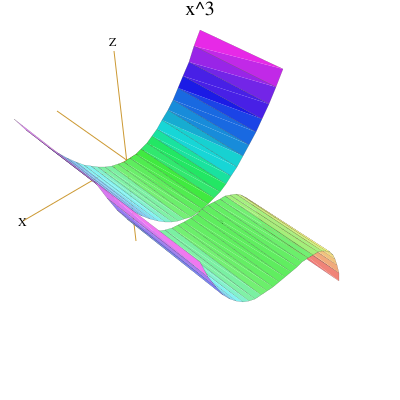
Unless you moved the original viewport, the new viewport covers the old one. You might want to check that the old object is still there by moving the top window.
Let’s show quadrilateral polygon outlines on the ribbons and then enclose the ribbons in a box.
Show quadrilateral polygon outlines.
drawStyle(vp,"shade");outlineRender(vp,"on")
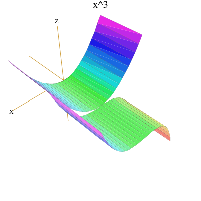
Enclose the ribbons in a box.
rotate(vp,20,-60); showRegion(vp,"on")
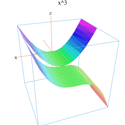
This process has become tedious! If we had to add two or three more ribbons, we would have to repeat the above steps several more times. It is time to write an interpreter program to help us take care of the details.
The above approach creates a new viewport for each additional ribbon. A better approach is to build one object composed of all ribbons before creating a viewport. To do this, use makeObject rather than draw. The operations have similar formats, but draw returns a viewport and makeObject returns a space object.
We now create a function drawRibbons of two arguments: flist, a list of formulas for the ribbons you want
to draw, and xrange, the range over which you want them drawn. Using this function, you can just
say
drawRibbons([x^2, x^3], x=-1..1)
to do all of the work required in the last section. Here is the drawRibbons program. Invoke your favorite editor and create a file called ribbon.input containing the following program.
1drawRibbons(flist, xrange) == 2 sp := createThreeSpace() -- Createemptyspacesp. 3 y0 := 0 --Theinitialribbonposition. 4 for f in flist repeat -- Foreachfunctionf, 5 makeObject(f, xrange, y=y0..y0+1, --createandaddaribbon 6 space==sp, var2Steps == 1) -- forftothespacesp. 7 y0 := y0 + 1 --Thenextribbonposition. 8 vp := makeViewport3D(sp, "Ribbons") -- Createviewport. 9 drawStyle(vp, "shade") --Selectshadingstyle. 10 outlineRender(vp, "on") -- Showpolygonoutlines. 11 showRegion(vp,"on") --Encloseinabox. 12 n := # flist -- Thenumberofribbons 13 zoom(vp,n,1,n) --Zoominx-andz-directions. 14 rotate(vp,0,75) -- Changetheangleofview. 15 vp --Returntheviewport. 16
Here are some remarks on the syntax used in the drawRibbons function (consult Chapter 6 for more details). Unlike most other programming languages which use semicolons, parentheses, or begin–end brackets to delineate the structure of programs, the structure of a FriCAS program is determined by indentation. The first line of a function definition always begins in column 1. All other lines of the function are indented with respect to the first line and form a pile (see Section 5.2 on page 248).
The definition of drawRibbons consists of a pile of expressions to be executed one after another. Each expression of the pile is indented at the same level. Lines 4-7 designate one single expression: since lines 5-7 are indented with respect to the others, these lines are treated as a continuation of line 4. Also since lines 5 and 7 have the same indentation level, these lines designate a pile within the outer pile.
The last line of a pile usually gives the value returned by the pile. Here it is also the value returned by the function. FriCAS knows this is the last line of the function because it is the last line of the file. In other cases, a new expression beginning in column one signals the end of a function.
The line drawStyle(vp,"shade") is given after the viewport has been created to select the drawing style. We
have also used the zoom option. Without the zoom, the viewport region would be scaled equally in all three
coordinate directions.
Let’s try the function drawRibbons. First you must read the file to give FriCAS the function definition.
Read the input file.
)read ribbon
Draw ribbons for  for

drawRibbons([x^i for i in 1..5],x=-1..1)
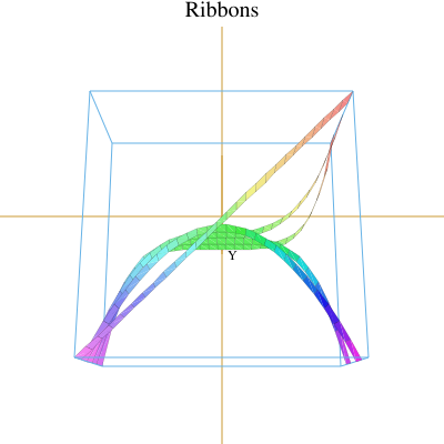
Before leaving the ribbon example, we make two improvements. Normally, the color given to each point in the space is a function of its height within a bounding box. The points at the bottom of the box are red, those at the top are purple.
To change the normal coloring, you can give an option colorFunction == function. When FriCAS goes about
displaying the data, it determines the range of colors used for all points within the box. FriCAS then
distributes these numbers uniformly over the number of hues. Here we use the simple color function
 for the
 ribbon.
Also, we add an argument yrange so you can give the range of y occupied by the ribbons. For example, if the
yrange is given as y=0..1 and there are  ribbons to be displayed, each ribbon would have width
 and
would appear in the range
 .
Refer to lines 4-9. Line 4 assigns to yVar the variable part of the yrange (after all, it need not be y). Suppose
that yrange is given as t = a..b where a and b have numerical values. Then line 5 assigns the value of a to the
variable y0. Line 6 computes the width of the ribbon by dividing the difference of a and b by the number,
num, of ribbons. The result is assigned to the variable width. Note that in the for-loop in line 7, we are
iterating in parallel; it is not a nested loop.
1drawRibbons(flist, xrange, yrange) == 2 sp := createThreeSpace() -- Createemptyspacesp. 3 num := # flist --Thenumberofribbons. 4 yVar := variable yrange -- Theribbonvariable. 5 y0:Float := low segment yrange --Thefirstribboncoordinate. 6 width:Float := (high segment yrange - y0)/num-- Thewidthofaribbon. 7 for f in flist for color in 1..num repeat --Foreachfunctionf, 8 makeObject(f, xrange, yVar = y0..y0+width, -- createandaddribbonto 9 var2Steps == 1, _ --spofadifferentcolor. 10 colorFunction == (x,y) +-> color, _ 11 space == sp) 12 y0 := y0 + width -- Thenextribboncoordinate. 13 vp := makeViewport3D(sp, "Ribbons") --Createviewport. 14 drawStyle(vp, "shade") -- Selectshadingstyle. 15 outlineRender(vp, "on") --Showpolygonoutlines. 16 showRegion(vp, "on") -- Enclose–inabox. 17 vp --Returntheviewport. 18
What you have seen so far is a high-level program using the graphics facility. We now turn to the more basic
notions of points, lines, and curves in three-dimensional graphs. These facilities use small floats (objects of
type DoubleFloat) for data. Let us first give names to the small float values  and
 . The small float
0.
zero := 0.0@DFLOAT
DoubleFloat The small float 1.
one := 1.0@DFLOAT
DoubleFloat The “@” sign means “of the type.” Thus zero is  of the type DoubleFloat. You can also say
0.0::DFLOAT.
Points can have four small float components:  coordinates and an optional color. A “curve” is simply a
list of points connected by straight line segments. Create the point
origin with color zero, that is, the
lowest color on the color map.
origin := point [zero,zero,zero,zero]
Point(DoubleFloat) Create the point unit with color zero.
unit := point [one,one,one,zero]
Point(DoubleFloat) Create the curve (well, here, a line) from origin to unit.
line := [origin, unit]
We make this line segment into an arrow by adding an arrowhead. The arrowhead extends to, say, p3 on the
left, and to, say, p4 on the right. To describe an arrow, you tell FriCAS to draw the two curves [p1, p2, p3]
and [p2, p4]. We also decide through experimentation on values for arrowScale, the ratio of the size of the
arrowhead to the stem of the arrow, and arrowAngle, the angle between the arrowhead and the
arrow.
Invoke your favorite editor and create an input file called arrows.input. This input file first defines the values
of arrowAngle and arrowScale, then defines the function makeArrow to draw an arrow from point
 to
 .
1arrowAngle := %pi-%pi/10.0@DFLOAT --Theangleofthe arrowhead. 2arrowScale := 0.2@DFLOAT --Thesizeofthe arrowhead 3 --relativetothe stem. 4makeArrow(p1, p2) == 5 delta := p2 - p1 --The arrow. 6 len := arrowScale * length delta -- Thelengthofthearrowhead. 7 theta := atan(delta.1, delta.2) --Theanglefromthe x-axis 8 c1 := len*cos(theta + arrowAngle) --Thex-coordofleft endpoint. 9 s1 := len*sin(theta + arrowAngle) -- They-coordofleftendpoint. 10 c2 := len*cos(theta - arrowAngle) --Thex-coordofright endpoint. 11 s2 := len*sin(theta - arrowAngle) -- They-coordofrightendpoint. 12 z := p2.3*(1 - arrowScale) --Thez-coordofboth endpoints. 13 p3 := point [p2.1 + c1, p2.2 + s1, z, p2.4] -- Theleftendpointofhead. 14 p4 := point [p2.1 + c2, p2.2 + s2, z, p2.4] --Therightendpointof head. 15 [[p1, p2, p3], [p2, p4]] --Thearrowasalistofcurves. 16
Read the file and then create an arrow from the point origin to the point unit. Read the input file defining
makeArrow.
)read arrows
Construct the arrow (a list of two curves).
arrow := makeArrow(origin,unit)
Compiling function makeArrow with type (Point(DoubleFloat), Point(DoubleFloat)) -> List(List(Point(DoubleFloat)))
List(List(Point(DoubleFloat))) Create an empty object sp of type ThreeSpace.
sp := createThreeSpace()
ThreeSpace(DoubleFloat) Add each curve of the arrow to the space sp.
for a in arrow repeat sp := curve(sp,a)
Create a three-dimensional viewport containing that space.
vp := makeViewport3D(sp,"Arrow")
Here is a better viewing angle.
rotate(vp,200,-60)
Let’s draw a “bouquet” of arrows. Each arrow is identical. The arrowheads are uniformly placed on a circle
parallel to the  -plane. Thus the position of each arrow differs only by the angle
 ,
 , between
the arrow and the
 -axis on the
 -plane.
Our bouquet is rather special: each arrow has a different color. This is arranged by letting the color of each
successive arrow be denoted by  . In this way, the color of arrows ranges from red to green to violet. Here is
a program to draw a bouquet of
 arrows.
1drawBouquet(n,title) == 2 z := 0.0@DFLOAT 3 e := 1.0@DFLOAT 4 angle := z -- Theinitialangle. 5 sp := createThreeSpace() --Createemptyspacesp. 6 for i in 0..n-1 repeat -- Foreachindexi,create: 7 start := point [z,z,z,angle] --pointatbaseofarrow; 8 end := point [cos angle, sin angle, e, angle] -- pointattipofarrow; 9 arrow := makeArrow(start,end) --itharrow. 10 for a in makeArrow(start,end) repeat -- Foreacharrowcomponent, 11 curve(sp,a) --addthecomponentto sp. 12 angle := angle + 2*%pi/n --Thenextangle. 13 makeViewport3D(sp,title) -- Createtheviewportfromsp. 14
Read the input file.
)read bouquet
A bouquet of a dozen arrows.
drawBouquet(12,"A Dozen Arrows")
We now put our arrows to good use drawing complex vector fields. These vector fields give a representation of
complex-valued functions of complex variables. Consider a Cartesian coordinate grid of points  in the
plane, and some complex-valued function
 defined on this grid. At every point on this grid,
compute the value of
 and call it
 . Since
 has both a real and imaginary value
for a given
 grid point, there are four dimensions to plot. What do we do? We represent
the values of
 by arrows planted at each grid point. Each arrow represents the value of
 in
polar coordinates
 . The length of the arrow is proportional to
 . Its direction is given by
 .
The code for drawing vector fields is in the file vectors.input. We discuss its contents from top to bottom.
Before showing you the code, we have two small matters to take care of. First, what if the function has large
spikes, say, ones that go off to infinity? We define a variable clipValue for this purpose. When
r exceeds the value of clipValue, then the value of clipValue is used instead of that for r.
For convenience, we define a function clipFun(x) which uses clipValue to “clip” the value of
x.
1clipValue : DFLOAT := 6 --Maximumvalue allowed. 2clipFun(x) == min(max(x,-clipValue),clipValue) 3
Notice that we identify clipValue as a small float but do not declare the type of the function clipFun. As it
turns out, clipFun is called with a small float value. This declaration ensures that clipFun never does a
conversion when it is called.
The second matter concerns the possible “poles” of a function, the actual points where the spikes have infinite
values. FriCAS uses normal DoubleFloat arithmetic which does not directly handle infinite values. If your
function has poles, you must adjust your step size to avoid landing directly on them (FriCAS calls error when
asked to divide a value by 0, for example).
We set the variables realSteps and imagSteps to hold the number of steps taken in the real and imaginary
directions, respectively. Most examples will have ranges centered around the origin. To avoid a pole at the
origin, the number of points is taken to be odd.
1realSteps: INT := 25 --Numberofreal steps. 2imagSteps: INT := 25 --Numberofimaginarysteps. 3)read arrows 4
Now define the function drawComplexVectorField to draw the arrows. It is good practice to declare the type of the main function in the file. This one declaration is usually sufficient to ensure that other lower-level functions are compiled with the correct types.
5C := Complex DoubleFloat 6S := Segment DoubleFloat 7drawComplexVectorField: (C -> C, S, S) -> VIEW3D 8
The first argument is a function mapping complex small floats into complex small floats. The second and third
arguments give the range of real and imaginary values as segments like a..b. The result is a three-dimensional
viewport. Here is the full function definition:
1drawComplexVectorField(f, realRange,imagRange) == 2 delReal := (high(realRange)-low(realRange))/realSteps -- Therealstepsize. 3 delImag := (high(imagRange)-low(imagRange))/imagSteps --Theimaginarystep size. 4 sp := createThreeSpace() --Createemptyspacesp. 5 real := low(realRange) -- Theinitialrealvalue. 6 for i in 1..realSteps+1 repeat --Beginrealiteration. 7 imag := low(imagRange) -- Theinitialimaginaryvalue. 8 for j in 1..imagSteps+1 repeat --Beginimaginaryiteration. 9 z := f complex(real,imag) -- Thevalueoffatthepoint. 10 arg := argument z --Thedirectionofthe arrow. 11 len := clipFun sqrt norm z --Thelengthofthearrow. 12 p1 := point [real, imag, 0.0@DFLOAT, arg] -- Thebasepointofthearrow. 13 scaleLen := delReal * len --Thescaledlengthof thearrow. 14 p2 := point [p1.1 + scaleLen*cos(arg), --Thetippointofthearrow. 15 p1.2 + scaleLen*sin(arg),0.0@DFLOAT, arg] 16 arrow := makeArrow(p1, p2) -- Createthearrow. 17 for a in arrow repeat curve(sp, a) --Addarrowtothespacesp. 18 imag := imag + delImag -- Thenextimaginaryvalue. 19 real := real + delReal --Thenextrealvalue. 20 makeViewport3D(sp, "Complex Vector Field") -- Drawit! 21
As a first example, let us draw f(z)== sin(z). There is no need to create a user function: just pass the sin
from Complex DoubleFloat. Read the file.
)read vectors
Draw the complex vector field of sin(x).
drawComplexVectorField(sin,-2..2,-2..2)
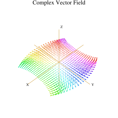
Here is another way to graph a complex function of complex arguments. For each complex value  ,
compute
 , again expressing the value in polar coordinates
 . We draw the complex
valued function, again considering the
 -plane as the complex plane, using
 as the height
(or
 -coordinate) and
 as the color. This is a standard plot—we learned how to do this in
Chapter 7—but here we write a new program to illustrate the creation of polygon meshes, or
grids.
Call this function drawComplex. It displays the points using the “mesh” of points. The function definition is in three parts.
1drawComplex: (C -> C, S, S) -> VIEW3D 2drawComplex(f, realRange, imagRange) == -- Thefirstpart. 3 delReal := (high(realRange)-low(realRange))/realSteps --Therealstepsize. 4 delImag := (high(imagRange)-low(imagRange))/imagSteps -- Theimaginarystepsize. 5 llp:List List Point DFLOAT := [] --Initiallistoflistofpoints llp. 6
Variables delReal and delImag give the step sizes along the real and imaginary directions as
computed by the values of the global variables realSteps and imagSteps. The mesh is represented
by a list of lists of points llp, initially empty. Now [ ] alone is ambiguous, so to set this initial
value you have to tell FriCAS what type of empty list it is. Next comes the loop which builds
llp.
1 real := low(realRange) --Theinitialreal value. 2 for i in 1..realSteps+1 repeat --Beginreal iteration. 3 imag := low(imagRange) --The initialimaginaryvalue. 4 lp := []$(List Point DFLOAT) --Theinitiallistofpoints lp. 5 for j in 1..imagSteps+1 repeat -- Beginimaginaryiteration. 6 z := f complex(real,imag) --Thevalueoffatthe point. 7 pt := point [real,imag, clipFun sqrt norm z, -- Createapoint. 8 argument z] 9 lp := cons(pt,lp) -- Addthepointtolp. 10 imag := imag + delImag --Thenextimaginary value. 11 real := real + delReal --Thenextreal value. 12 llp := cons(lp, llp) --Addlptollp. 13
The code consists of both an inner and outer loop. Each pass through the inner loop adds one list lp of points
to the list of lists of points llp. The elements of lp are collected in reverse order.
1 makeViewport3D(mesh(llp), "Complex Function") --Createameshanddisplay. 2
The operation mesh then creates an object of type ThreeSpace(DoubleFloat) from the list of lists of points. This is then passed to makeViewport3D to display the image.
Now add this function directly to your vectors.input file and re-read the file using )read vectors. We try
drawComplex using a user-defined function f.
Read the file.
)read vectors
This one has a pole at  .
f(z) == exp(1/z)
Draw it with an odd number of steps to avoid the pole.
drawComplex(f,-2..2,-2..2)
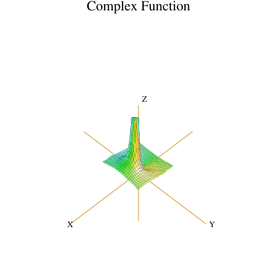
In Section 6.14 on page 335, you learned how to use the operation function to create a function from symbolic formulas. Here we introduce a similar operation which not only creates functions, but functions from functions.
The facility we need is provided by the package MakeUnaryCompiledFunction(E,S,T). This package
produces a unary (one-argument) compiled function from some symbolic data generated by a previous
computation.1
The E tells where the symbolic data comes from; the S and T give FriCAS the source and target type of the
function, respectively. The compiled function produced has type S . To produce a compiled function
with definition  T
p(x)== expr, call compiledFunction(expr, x) from this package. The function you get
has no name. You must assign the function to the variable p to give it that name. Do some
computation.
(x+1/3)^5
Polynomial(Fraction(Integer)) Convert this to an anonymous function of x. Assign it to the variable p to give the
function a name.
p := compiledFunction(%,x)$MakeUnaryCompiledFunction(POLY FRAC INT,DFLOAT,DFLOAT)
Compiling function %A with type DoubleFloat -> DoubleFloat
(DoubleFloat -> DoubleFloat) Apply the function.
p(sin(1.3))
For a more sophisticated application, read on.
We resume our continuing saga of arrows and complex functions. Suppose we want to investigate the behavior
of Newton’s iteration function in the complex plane. Given a function  , we want to find the complex values
 such that
 .
The first step is to produce a Newton iteration formula for a given  :
 We represent
this formula by a function
 that performs the computation on the right-hand side, that is,
 .
The type Expression Integer (abbreviated EXPR INT) is used to represent general symbolic expressions
in FriCAS. To make our facility as general as possible, we assume  has this type. Given
 , we want to
produce a Newton iteration function
g which, given a complex point  , delivers the next Newton iteration
point
 .
This time we write an input file called newton.input. We need to import MakeUnaryCompiledFunction
(discussed in the last section), call it with appropriate types, and then define the function newtonStep which
references it. Here is the function newtonStep:
1C := Complex DoubleFloat --Thecomplexnumbers. 2E := Expression Integer -- Theexpressiondomain. 3complexFunPack:=MakeUnaryCompiledFunction(E,C,C) --Packageformaking functions. 4 5newtonStep(f) == --Newton’siterationfunction. 6 fun := complexNumericFunction f -- Functionfor. 7 deriv := complexDerivativeFunction(f,1) --Functionfor
. 8 (x:C):C +-> -- Returntheiteratorfunction. 9 x - fun(x)/deriv(x) 10 11complexNumericFunction f == -- Turnanexpressionfintoa 12 v := theVariableIn f --function. 13 compiledFunction(f, v)$complexFunPack 14 15complexDerivativeFunction(f,n) == -- Createannthderivative 16 v := theVariableIn f --function. 17 df := D(f,v,n) 18 compiledFunction(df, v)$complexFunPack 19 20theVariableIn f == -- Returnsthevariablein
. 21 vl := variables f --Thelistofvariables. 22 nv := # vl -- Thenumberofvariables. 23 nv > 1 => error "Expression is not univariate." 24 nv = 0 => ’x -- Returnadummyvariable. 25 first vl 26
Do you see what is going on here? A formula f is passed into the function newtonStep. First, the function
turns f into a compiled program mapping complex numbers into complex numbers. Next, it does the same
thing for the derivative of f. Finally, it returns a function which computes a single step of Newton’s
iteration.
The function complexNumericFunction extracts the variable from the expression f and then turns f into a
function which maps complex numbers into complex numbers. The function complexDerivativeFunction
does the same thing for the derivative of f. The function theVariableIn extracts the variable from the
expression f, calling the function error if f has more than one variable. It returns the dummy variable x if f
has no variables.
Let’s now apply newtonStep to the formula for computing cube roots of two. Read the input file with the definitions.
)read newton
)read vectors
The cube root of two.
f := x^3 - 2
Polynomial(Integer) Get Newton’s iteration formula.
g := newtonStep f
Compiling function theVariable with type Polynomial(Integer) -> Symbol
Compiling function complexNumericFunction with type Polynomial(Integer) -> ( Complex(DoubleFloat) -> Complex(DoubleFloat))
Compiling function complexDerivativeFunction with type (Polynomial(Integer), PositiveInteger) -> (Complex(DoubleFloat) -> Complex(DoubleFloat))
Compiling function newtonStep with type Polynomial(Integer) -> (Complex( DoubleFloat) -> Complex(DoubleFloat))
Compiling function %B with type Complex(DoubleFloat) -> Complex(DoubleFloat)
Compiling function %C with type Complex(DoubleFloat) -> Complex(DoubleFloat)
(Complex(DoubleFloat) -> Complex(DoubleFloat)) Let a denote the result of applying Newton’s iteration once to the complex number
1 + %i.
a := g(1.0 + %i)
Complex(DoubleFloat) Now apply it repeatedly. How fast does it converge?
[(a := g(a)) for i in 1..]
Stream(Complex(DoubleFloat)) Check the accuracy of the last iterate.
a^3
In ‘MappingPackage1’ on page 1104, we show how functions can be manipulated as objects in FriCAS. A
useful operation to consider here is *, which means composition. For example g*g causes the Newton
iteration formula to be applied twice. Correspondingly, g^n means to apply the iteration formula n
times.
Apply g twice to the point 1 + %i.
(g*g) (1.0 + %i)
Complex(DoubleFloat) Apply g 11 times.
(g^11) (1.0 + %i)
Look now at the vector field and surface generated after two steps of Newton’s formula for the cube root of two. The poles in these pictures represent bad starting values, and the flat areas are the regions of convergence to the three roots. The vector field.
drawComplexVectorField(g^3,-3..3,-3..3)
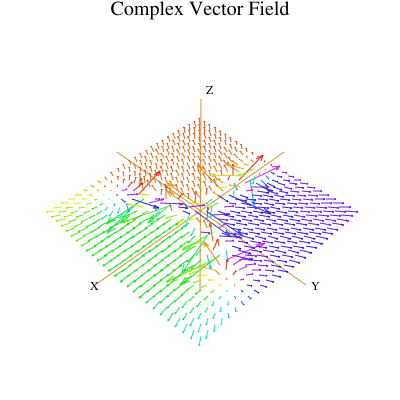
The surface.
drawComplex(g^3,-3..3,-3..3)
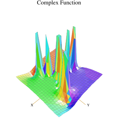
Packages provide the bulk of FriCAS’s algorithmic library, from numeric packages for computing special functions to symbolic facilities for differential equations, symbolic integration, and limits.
In Chapter 10, we developed several useful functions for drawing vector fields and complex functions. We now show you how you can add these functions to the FriCAS library to make them available for general use.
The way we created the functions in Chapter 10 is typical of how you, as an advanced FriCAS user, may interact with FriCAS. You have an application. You go to your editor and create an input file defining some functions for the application. Then you run the file and try the functions. Once you get them all to work, you will often want to extend them, add new features, perhaps write additional functions.
Eventually, when you have a useful set of functions for your application, you may want to add them to your local FriCAS library. To do this, you embed these function definitions in a package and add that package to the library.
To introduce new packages, categories, and domains into the system, you need to use the FriCAS compiler to convert the constructors into executable machine code. An existing compiler in FriCAS is available on an “as-is” basis. A new, faster compiler will be available in version 2.0 of FriCAS.
1C ==> Complex DoubleFloat -- Allconstructorsusedinafile 2S ==> Segment DoubleFloat --mustbespelledout infull 3INT ==> Integer --unlessabbreviatedbymacros 4DFLOAT ==> DoubleFloat -- liketheseatthetopof 5VIEW3D ==> ThreeDimensionalViewport --afile. 6CURVE ==> List List Point DFLOAT 7 8)abbrev package DRAWCX DrawComplex -- Identifykindsandabbreviations 9DrawComplex(): Exports == Implementation where --Typedefinition beginshere. 10 11 Exports == with --Exportpartbegins. 12 drawComplex: (C -> C,S,S,Boolean) -> VIEW3D -- ExportedOperations 13 drawComplexVectorField: (C -> C,S,S) -> VIEW3D 14 setRealSteps: INT -> INT 15 setImagSteps: INT -> INT 16 setClipValue: DFLOAT -> DFLOAT 17 18 Implementation == add -- Implementationpartbegins. 19 arrowScale : DFLOAT := (0.2)::DFLOAT --(relativesize)Local variable1. 20 arrowAngle : DFLOAT := pi()-pi()/(20::DFLOAT) --Localvariable2. 21 realSteps : INT := 11 -- (realsteps)Localvariable3. 22 imagSteps : INT := 11 --(imaginarysteps)Local variable4. 23 clipValue : DFLOAT := 10::DFLOAT --(maximumvectorlength)Localvariable 5. 24 25 setRealSteps(n) == realSteps := n --Exportedfunctiondefinition1. 26 setImagSteps(n) == imagSteps := n -- Exportedfunctiondefinition2. 27 setClipValue(c) == clipValue := c --Exportedfunction definition3. 28 29 clipFun: DFLOAT -> DFLOAT --Cliplargemagnitudes. 30 clipFun(x) == min(max(x, -clipValue), clipValue) -- Localfunctiondefinition1. 31 32 makeArrow: (Point DFLOAT,Point DFLOAT,DFLOAT,DFLOAT) -> CURVE 33 makeArrow(p1, p2, len, arg) == ... -- Localfunctiondefinition2. 34 35 drawComplex(f, realRange, imagRange, arrows?) == ... --Exportedfunction definition4. 36
Each package has a name and an abbreviation. For a package of the complex draw functions from Chapter 10, we choose the name DrawComplex and abbreviation DRAWCX.1 To be sure that you have not chosen a name or abbreviation already used by the system, issue the system command )show for both the name and the abbreviation.
Once you have named the package and its abbreviation, you can choose any new filename you like with extension “.spad” to hold the definition of your package. We choose the name drawpak.spad. If your application involves more than one package, you can put them all in the same file. FriCAS assumes no relationship between the name of a library file, and the name or abbreviation of a package.
Near the top of the “.spad” file, list all the abbreviations for the packages using )abbrev, each command beginning in column one. Macros giving names to FriCAS expressions can also be placed near the top of the file. The macros are only usable from their point of definition until the end of the file.
Consider the definition of DrawComplex in Figure 11.1. After the macro definition
S ==> Segment DoubleFloat
the name S can be used in the file as a shorthand for Segment DoubleFloat.2 The abbreviation command for the package
)abbrev package DRAWCX DrawComplex
is given after the macros (although it could precede them).
The definition of a package has the syntax:
PackageForm : Exports == Implementation
The syntax for defining a package constructor is the same as that for defining any function in FriCAS. In
practice, the definition extends over many lines so that this syntax is not practical. Also, the type of a package
is expressed by the operator with followed by an explicit list of operations. A preferable way to write the
definition of a package is with a where expression:
The definition of a package usually has the form:
PackageForm : Exports == Implementation where
optional type declarations
Exports == with
list of exported operations
Implementation == add
list of function definitions for exported operations
The DrawComplex package takes no parameters and exports five operations, each a separate item of a pile. Each operation is described as a declaration: a name, followed by a colon (“:”), followed by the type of the operation. All operations have types expressed as mappings with the syntax
source 
A constructor as defined in FriCAS is called an abstract datatype in the computer science literature. Abstract datatypes separate “specification” (what operations are provided) from “implementation” (how the operations are implemented). The Exports (specification) part of a constructor is said to be “public” (it provides the user interface to the package) whereas the Implementation part is “private” (information here is effectively hidden—programs cannot take advantage of it).
The Exports part specifies what operations the package provides to users. As an author of a package, you must ensure that the Implementation part provides a function for each operation in the Exports part.3
An important difference between interactive programming and the use of packages is in the handling of global
variables such as realSteps and imagSteps. In interactive programming, you simply change the values of
variables by assignment. With packages, such variables are local to the package—their values can only be set
using functions exported by the package. In our example package, we provide two functions setRealSteps and
setImagSteps for this purpose.
Another local variable is clipValue which can be changed using the exported operation setClipValue. This
value is referenced by the internal function clipFun that decides whether to use the computed value of the
function at a point or, if the magnitude of that value is too large, the value assigned to clipValue (with the
appropriate sign).
The part to the right of add in the Implementation part of the definition is called a capsule. The purpose of a capsule is:
What is a local environment? First, what is an environment? Think of the capsule as an input file that
FriCAS reads from top to bottom. Think of the input file as having a )clear all at the top so that initially
no variables or functions are defined. When this file is read, variables such as realSteps and arrowSize in
DrawComplex are set to initial values. Also, all the functions defined in the capsule are compiled. These
include those that are exported (like drawComplex), and those that are not (like makeArrow). At the end, you
get a set of name-value pairs: variable names (like realSteps and arrowSize) are paired with
assigned values, while operation names (like drawComplex and makeArrow) are paired with function
values.
This set of name-value pairs is called an environment. Actually, we call this environment the “initial environment” of a package: it is the environment that exists immediately after the package is first built. Afterwards, functions of this capsule can access or reset a variable in the environment. The environment is called local since any changes to the value of a variable in this environment can be seen only by these functions.
Only the functions from the package can change the variables in the local environment. When two functions are called successively from a package, any changes caused by the first function called are seen by the second.
Since the environment is local to the package, its names don’t get mixed up with others in the system or your
workspace. If you happen to have a variable called realSteps in your workspace, it does not affect what the
DrawComplex functions do in any way.
The functions in a package are compiled into machine code. Unlike function definitions in input files that may be compiled repeatedly as you use them with varying argument types, functions in packages have a unique type (generally parameterized by the argument parameters of a package) and a unique compilation residing on disk.
The capsule itself is turned into a compiled function. This so-called capsule function is what builds the initial environment spoken of above. If the package has arguments (see below), then each call to the package constructor with a distinct pair of arguments builds a distinct package, each with its own local environment.
A good question at this point would be “Is writing a package more difficult than writing an input file?”
The programs in input files are designed for flexibility and ease-of-use. FriCAS can usually work out all of your types as it reads your program and does the computations you request. Let’s say that you define a one-argument function without giving its type. When you first apply the function to a value, this value is understood by FriCAS as identifying the type for the argument parameter. Most of the time FriCAS goes through the body of your function and figures out the target type that you have in mind. FriCAS sometimes fails to get it right. Then—and only then—do you need a declaration to tell FriCAS what type you want.
Input files are usually written to be read by FriCAS—and by you. Without suitable documentation and declarations, your input files are likely incomprehensible to a colleague—and to you some months later!
Packages are designed for legibility, as well as run-time efficiency. There are few new concepts you need to learn to write packages. Rather, you just have to be explicit about types and type conversions. The types of all functions are pre-declared so that FriCAS—and the reader— knows precisely what types of arguments can be passed to and from the functions (certainly you don’t want a colleague to guess or to have to work this out from context!). The types of local variables are also declared. Type conversions are explicit, never automatic.4
In summary, packages are more tedious to write than input files. When writing input files, you can casually go ahead, giving some facts now, leaving others for later. Writing packages requires forethought, care and discipline.
Once you have defined the package DrawComplex, you need to compile and test it. To compile the package, issue the system command )compile drawpak. FriCAS reads the file drawpak.spad and compiles its contents into machine binary. If all goes well, the file DRAWCX.NRLIB is created in your local directory for the package. To test the package, you must load the package before trying an operation.
Compile the package.
)compile drawpak
Expose the package.
)expose DRAWCX
DrawComplex is now explicitly exposed in frame initial
Use an odd step size to avoid a pole at the origin.
setRealSteps 51
setImagSteps 51
PositiveInteger Define f to be the Gamma function.
f(z) == Gamma(z)
Clip values of function with magnitude larger than 7.
setClipValue 7
DoubleFloat Draw the Gamma function.
drawComplex(f,-%pi..%pi,-%pi..%pi, false)
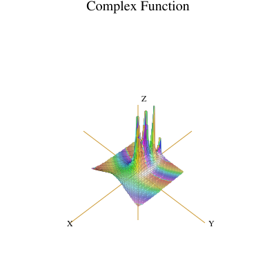
The power of packages becomes evident when packages have parameters. Usually these parameters are domains and the exported operations have types involving these parameters.
In Chapter 2, you learned that categories denote classes of domains. Although we cover this notion in detail in the next chapter, we now give you a sneak preview of its usefulness.
In Section 6.15 on page 342, we defined functions bubbleSort(m) and insertionSort(m) to sort a list of
integers. If you look at the code for these functions, you see that they may be used to sort any structure m
with the right properties. Also, the functions can be used to sort lists of any elements—not just integers. Let
us now recall the code for bubbleSort.
bubbleSort(m) == n := #m for i in 1..(n-1) repeat for j in n..(i+1) by -1 repeat if m.j < m.(j-1) then swap!(m,j,j-1) m
What properties of “lists of integers” are assumed by the sorting algorithm? In the first line,
the operation # computes the maximum index of the list. The first obvious property is that m
must have a finite number of elements. In FriCAS, this is done by telling FriCAS that m has the
category finiteAggregate. As we show later in Section 12.9 on page 1480, by using category tests
programs can query domains as to the presence or absence of property (attribute) represented by a
category.
The operation swap! swaps elements of m. Using Browse, you find that swap! requires its elements to come
from a domain of category IndexedAggregate which also has category shallowlyMutable. This category
means that you can change the internal components of m without changing its external structure.
Shallowly-mutable data structures include lists, streams, one- and two-dimensional arrays, vectors, and
matrices.
The category IndexedAggregate designates the class of aggregates whose elements can be accessed by the
notation m(s) for suitable selectors s. The category IndexedAggregate takes two arguments: Index, a
domain of selectors for the aggregate, and Entry, a domain of entries for the aggregate. Since the
sort functions access elements by integers, we must choose Index = Integer. The most general
class of domains for which bubbleSort and insertionSort are defined are those of category
IndexedAggregate(Integer,Entry) with the two additional categories shallowlyMutable and
finiteAggregate.
Using Browse, you can also discover that FriCAS has many kinds of domains of category shallowlyMutable. Those of class IndexedAggregate(Integer,Entry) include Bits, FlexibleArray, OneDimensionalArray, List, String, and Vector, and also HashTable and EqTable with integer keys. Although you may never want to sort all such structures, we nonetheless demonstrate FriCAS’s ability to do so.
Another requirement is that Entry has an operation <. One way to get this operation is to assume that
Entry has category OrderedSet. By definition, it will then export a < operation. A more general approach is
to allow any comparison function f to be used for sorting. This function will be passed as an argument to the
sorting functions.
Our sorting package then takes two arguments: a domain S of objects of any type, and a domain A, an
aggregate of type IndexedAggregate(Integer, S) with the above two additional categories. Here is its
definition using what are close to the original definitions of bubbleSort and insertionSort for sorting lists
of integers. The symbol “!” is added to the ends of the operation names. This uniform naming
convention is used for FriCAS operation names that destructively change one or more of their
arguments.
1SortPackage(S,A) : Exports == Implementation where 2 S: Object 3 A: IndexedAggregate(Integer,S) 4 with (finiteAggregate; shallowlyMutable) 5 6 Exports == with 7 bubbleSort!: (A,(S,S) -> Boolean) -> A 8 insertionSort!: (A, (S,S) -> Boolean) -> A 9 10 Implementation == add 11 bubbleSort!(m,f) == 12 n := #m 13 for i in 1..(n-1) repeat 14 for j in n..(i+1) by -1 repeat 15 if f(m.j,m.(j-1)) then swap!(m,j,j-1) 16 m 17 insertionSort!(m,f) == 18 for i in 2..#m repeat 19 j := i 20 while j > 1 and f(m.j,m.(j-1)) repeat 21 swap!(m,j,j-1) 22 j := (j - 1) pretend PositiveInteger 23 m 24
When packages have parameters, you can say that an operation is or is not exported depending on the values
of those parameters. When the domain of objects S has an < operation, we can supply one-argument versions
of bubbleSort and insertionSort which use this operation for sorting. The presence of the operation < is
guaranteed when S is an ordered set.
1Exports == with 2 bubbleSort!: (A,(S,S) -> Boolean) -> A 3 insertionSort!: (A, (S,S) -> Boolean) -> A 4 5 if S has OrderedSet then 6 bubbleSort!: A -> A 7 insertionSort!: A -> A 8
In addition to exporting the one-argument sort operations conditionally, we must provide conditional
definitions for the operations in the Implementation part. This is easy: just have the one-argument functions
call the corresponding two-argument functions with the operation < from S.
1 Implementation == add 2 ... 3 if S has OrderedSet then 4 bubbleSort!(m) == bubbleSort!(m,<$S) 5 insertionSort!(m) == insertionSort!(m,<$S) 6
In Section 6.15 on page 342, we give an alternative definition of bubbleSort using first and rest that is
more efficient for a list (for which access to any element requires traversing the list from its first
node). To implement a more efficient algorithm for lists, we need the operation setelt! which
allows us to destructively change the first and rest of a list. Using Browse, you find that these
operations come from category UnaryRecursiveAggregate. Several aggregate types are unary
recursive aggregates including those of List and AssociationList. We provide two different
implementations for bubbleSort! and insertionSort!: one for list-like structures, another for array-like
structures.
1Implementation == add 2 ... 3 if A has UnaryRecursiveAggregate(S) then 4 bubbleSort!(m,fn) == 5 empty? m => m 6 l := m 7 while not empty? (r := l.rest) repeat 8 r := bubbleSort! r 9 x := l.first 10 if fn(r.first,x) then 11 l.first := r.first 12 r.first := x 13 l.rest := r 14 l := l.rest 15 m 16 insertionSort!(m,fn) == 17 ... 18
The ordering of definitions is important. The standard definitions come first and then the predicate
A has UnaryRecursiveAggregate(S)
is evaluated. If true, the special definitions cover up the standard ones.
Another equivalent way to write the capsule is to use an if-then-else expression:
1 if A has UnaryRecursiveAggregate(S) then 2 ... 3 else 4 ... 5
Once you have written the package, embed it in a file, for example, sortpak.spad. Be sure to include an
)abbrev command at the top of the file:
)abbrev package SORTPAK SortPackage
Now compile the file (using )compile sortpak.spad). Expose the constructor. You are then ready to begin testing.
)expose SORTPAK
SortPackage is now explicitly exposed in frame initial
Define a list.
l := [1,7,4,2,11,-7,3,2]
List(Integer) Since the integers are an ordered set, a one-argument operation will do.
bubbleSort!(l)
List(Integer) Re-sort it using “greater than.”
bubbleSort!(l,(x,y) +-> x > y)
List(Integer) Now sort it again using < on integers.
bubbleSort!(l, <$Integer)
List(Integer) A string is an aggregate of characters so we can sort them as well.
bubbleSort! "Mathematical Sciences"
String Is < defined on booleans?
false < true
Boolean Good! Create a bit string representing ten consecutive boolean values true.
u : Bits := new(10,true)
Bits Set bits 3 through 5 to false, then display the result.
u(3..5) := false; u
Bits Now sort these booleans.
bubbleSort! u
Bits Create an “eq-table” (see ‘EqTable’ on page 837), a table having integers as keys and strings as values.
t : EqTable(Integer,String) := table()
EqTable(Integer, String) Give the table a first entry.
t.1 := "robert"
String And a second.
t.2 := "richard"
String What does the table look like?
t
EqTable(Integer, String) Now sort it.
bubbleSort! t
Recall that packages as abstract datatypes are compiled independently and put into the library. The curious reader may ask: “How is the interpreter able to find an operation such as bubbleSort!? Also, how is a single compiled function such as bubbleSort! able to sort data of different types?”
After the interpreter loads the package SortPackage, the four operations from the package become known to the interpreter. Each of these operations is expressed as a modemap in which the type of the operation is written in terms of symbolic domains.
)expose SORTPAK
See the modemaps for bubbleSort!.
)display op bubbleSort!
There are 2 exposed functions called bubbleSort! : [1] (D1,((D3, D3) -> Boolean)) -> D1 from SortPackage(D3,D1) if D3 has TYPE and D1 has Join(IXAGG(INT,D3),ATFINAG,ATSHMUT) [2] D1 -> D1 from SortPackage(D2,D1) if D2 has ORDSET and D2 has TYPE and D1 has Join(IXAGG(INT,D2),ATFINAG ,ATSHMUT)
What happens if you ask for bubbleSort!([1,-5,3])? There is a unique modemap for an operation named
bubbleSort! with one argument. Since [1,-5,3] is a list of integers, the symbolic domain D1 is defined as
List(Integer). For some operation to apply, it must satisfy the predicate for some D2. What D2? The third
expression of the and requires D1 has IndexedAggregate(Integer, D2) with two additional categories. So
the interpreter searches for an IndexedAggregate among the ancestors of List (Integer) (see Section 12.4
on page 1475). It finds one: IndexedAggregate(Integer, Integer). The interpreter tries defining D2 as
Integer. After substituting for D1 and D2, the predicate evaluates to true. An applicable operation has been
found!
Now FriCAS builds the package SortPackage(List(Integer), Integer). According to its definition, this
package exports the required operation: bubbleSort!: List Integer
[1,-5,3]. The bubbleSort! function is executed in its local environment and produces the
result.
This chapter unravels the mysteries of categories—what they are, how they are related to domains and packages, how they are defined in FriCAS, and how you can extend the system to include new categories of your own.
We assume that you have read the introductory material on domains and categories in Section 2.1.1 on page 132. There you learned that the notion of packages covered in the previous chapter are special cases of domains. While this is in fact the case, it is useful here to regard domains as distinct from packages.
Think of a domain as a datatype, a collection of objects (the objects of the domain). From your “sneak preview” in the previous chapter, you might conclude that categories are simply named clusters of operations exported by domains. As it turns out, categories have a much deeper meaning. Categories are fundamental to the design of FriCAS. They control the interactions between domains and algorithmic packages, and, in fact, between all the components of FriCAS.
Categories form hierarchies as shown on the inside cover pages of this book. The inside front-cover pages illustrate the basic algebraic hierarchy of the FriCAS programming language. The inside back-cover pages show the hierarchy for data structures.
Think of the category structures of FriCAS as a foundation for a city on which superstructures (domains) are built. The algebraic hierarchy, for example, serves as a foundation for constructive mathematical algorithms embedded in the domains of FriCAS. Once in place, domains can be constructed, either independently or from one another.
Superstructures are built for quality—domains are compiled into machine code for run-time efficiency. You can extend the foundation in directions beyond the space directly beneath the superstructures, then extend selected superstructures to cover the space. Because of the compilation strategy, changing components of the foundation generally means that the existing superstructures (domains) built on the changed parts of the foundation (categories) have to be rebuilt—that is, recompiled.
Before delving into some of the interesting facts about categories, let’s see how you define them in FriCAS.
A category is defined by a function with exactly the same format as any other function in FriCAS.
The definition of a category has the syntax:
CategoryForm : Category == Extensions [ with Exports ]
The brackets [ ] here indicate optionality.
The first example of a category definition is SetCategory, the most basic of the algebraic categories in FriCAS.
1SetCategory(): Category == 2 Join(Type,CoercibleTo OutputForm) with 3 "=" : (%, %) -> Boolean 4
The definition starts off with the name of the category (SetCategory); this is always in column one in the source file. All parts of a category definition are then indented with respect to this first line.
In Chapter 2, we talked about Ring as denoting the class of all domains that are rings, in short, the class of all rings. While this is the usual naming convention in FriCAS, it is also common to use the word “Category” at the end of a category name for clarity. The interpretation of the name SetCategory is, then, “the category of all domains that are (mathematical) sets.”
The name SetCategory is followed in the definition by its formal parameters enclosed in parentheses “()”. Here there are no parameters. As required, the type of the result of this category function is the distinguished name Category.
Then comes the “==”. As usual, what appears to the right of the “==” is a definition, here, a
category definition. A category definition always has two parts separated by the reserved word
with.
The first part tells what categories the category extends. Here, the category extends two categories: Type, the category of all domains, and CoercibleTo(OutputForm). The operation Join is a system-defined operation that forms a single category from two or more other categories.
Every category other than Type is an extension of some other category. If, for example, SetCategory extended only the category Type, the definition here would read “Type with ...”. In fact, the Type is optional in this line; “with ...” suffices.
To the right of the with is a list of all the exports of the category. Each exported operation has a name and a
type expressed by a declaration of the form “name: type”.
Categories can export symbols, as well as 0 and 1 which denote domain constants.1 In the current implementation, all other exports are operations with types expressed as mappings with the syntax
source 
The category SetCategory has a single export: the operation = whose type is given by the mapping
(%, %). The “%” in a mapping type always means “the domain.” Thus the operation = takes two
arguments from the domain and returns a value of type Boolean.
 Boolean
The source part of the mapping here is given by a tuple consisting of two or more types separated by commas and enclosed in parentheses. If an operation takes only one argument, you can drop the parentheses around the source type. If the mapping has no arguments, the source part of the mapping is either left blank or written as “()”. Here are examples of formats of various operations with some contrived names.
someIntegerConstant : % aZeroArgumentOperation: () -> Integer aOneArgumentOperation: Integer -> % aTwoArgumentOperation: (Integer,%) -> Void aThreeArgumentOperation: (%,Integer,%) -> Fraction(%)
The definition of SetCategory above is missing an important component: its library documentation. Here is its definition, complete with documentation.
1++ Description: 2++ \spadtype{SetCategory} is the basic category 3++ for describing a collection of elements with 4++ \spadop{=} (equality) and a \spadfun{coerce} 5++ to \spadtype{OutputForm}. 6 7SetCategory(): Category == 8 Join(Type, CoercibleTo OutputForm) with 9 "=": (%, %) -> Boolean 10 ++ \spad{x = y} tests if \spad{x} and 11 ++ \spad{y} are equal. 12
Documentary comments are an important part of constructor definitions. Documentation is given both for the category itself and for each export. A description for the category precedes the code. Each line of the description begins in column one with “++”. The description starts with the word Description:.2 All lines of the description following the initial line are indented by the same amount.
Mark the name of any constructor (with or without parameters) with \spadtype like this
\spadtype{Polynomial(Integer)}
Similarly, mark an operator name with \spadop, a FriCAS operation (function) with \spadfun, and a variable or FriCAS expression with \spad. Library documentation is given in a TeX-like language so that it can be used both for hard-copy and for Browse. These different wrappings cause operations and types to have mouse-active buttons in Browse. For hard-copy output, wrapped expressions appear in a different font. The above documentation appears in hard-copy as:
SetCategory is the basic category for describing a collection of elements with = (equality) and a coerce to OutputForm.
and
x = ytests ifxandyare equal.
For our purposes in this chapter, we omit the documentation from further category descriptions.
A second example of a category is SemiGroup, defined by:
1SemiGroup(): Category == SetCategory with 2 "*": (%,%) -> % 3 "^": (%, PositiveInteger) -> % 4
This definition is as simple as that for SetCategory, except that there are two exported operations. Multiple exported operations are written as a pile, that is, they all begin in the same column. Here you see that the category mentions another type, PositiveInteger, in a signature. Any domain can be used in a signature.
Since categories extend one another, they form hierarchies. Each category other than Type has one or more
parents given by the one or more categories mentioned before the with part of the definition. SemiGroup
extends SetCategory and SetCategory extends both Type and CoercibleTo (OutputForm). Since
CoercibleTo (OutputForm) also extends Type, the mention of Type in the definition is unnecessary but
included for emphasis.
We say a category designates a class of domains. What class of domains? That is, how does FriCAS know what domains belong to what categories? The simple answer to this basic question is key to the design of FriCAS:
Domains belong to categories by assertion.
When a domain is defined, it is asserted to belong to one or more categories. Suppose, for example, that an author of domain
String wishes to use the binary operator * to denote concatenation. Thus "hello " * "there" would produce the string
"hello there"3.
The author of String could then assert that String is a member of SemiGroup. According to our definition
of SemiGroup, strings would then also have the operation ^ defined automatically. Then "--" ^ 4
would produce a string of eight dashes "--------". Since String is a member of SemiGroup, it
also is a member of SetCategory and thus has an operation = for testing that two strings are
equal.
Now turn to the algebraic category hierarchy inside the front cover of this book. Any domain that is a member of a category extending SemiGroup is a member of SemiGroup (that is, it is a semigroup). In particular, any domain asserted to be a Ring is a semigroup since Ring extends Monoid, that, in turn, extends SemiGroup. The definition of Integer in FriCAS asserts that Integer is a member of category IntegerNumberSystem, that, in turn, asserts that it is a member of EuclideanDomain. Now EuclideanDomain extends PrincipalIdealDomain and so on. If you trace up the hierarchy, you see that EuclideanDomain extends Ring, and, therefore, SemiGroup. Thus Integer is a semigroup and also exports the operations * and ^.
We actually omitted the last part of the definition of SemiGroup in Section 12.4 on page 1475. Here now is its complete FriCAS definition.
1SemiGroup(): Category == SetCategory with 2 "*": (%, %) -> % 3 "^": (%, PositiveInteger) -> % 4 add 5 import RepeatedSquaring(%) 6 x: % ^ n: PositiveInteger == expt(x,n) 7
The add part at the end is used to give “default definitions” for exported operations. Once you have a
multiplication operation *, you can define exponentiation for positive integer exponents using repeated
multiplication:
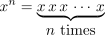
This definition for ^ is called a default definition. In general, a category can give default definitions for any operation it exports. Since SemiGroup and all its category descendants in the hierarchy export ^, any descendant category may redefine ^ as well.
A domain of category SemiGroup (such as Integer) may or may not choose to define its own ^ operation. If it does not, a default definition that is closest (in a “tree-distance” sense of the hierarchy) to the domain is chosen.
The part of the category definition following an “add” operation is a capsule, as discussed in the previous chapter. The line
import RepeatedSquaring(%)
references the package RepeatedSquaring(%), that is, the package RepeatedSquaring that takes “this domain” as its parameter. For example, if the semigroup Polynomial (Integer) does not define its own exponentiation operation, the definition used may come from the package RepeatedSquaring (Polynomial (Integer)). The next line gives the definition in terms of expt from that package.
The default definitions are collected to form a “default package” for the category. The name of the package is the same as the category but with an ampersand (“&”) added at the end. A default package always takes an additional argument relative to the category. Here is the definition of the default package SemiGroup& as automatically generated by FriCAS from the above definition of SemiGroup.
1SemiGroup_&(%): Exports == Implementation where 2 %: SemiGroup 3 Exports == with 4 "^": (%, PositiveInteger) -> % 5 Implementation == add 6 import RepeatedSquaring(%) 7 x:% ^ n:PositiveInteger == expt(x,n) 8
In the previous section you saw the complete FriCAS program defining SemiGroup. According to this definition, semigroups are sets with the operations * and ^.
You might ask: “Aside from the notion of default packages, isn’t a category just a macro, that is, a shorthand equivalent to the two operations * and ^ with their types?” If a category were a macro, every time you saw the word SemiGroup, you would rewrite it by its list of exported operations. Furthermore, every time you saw the exported operations of SemiGroup among the exports of a constructor, you could conclude that the constructor exported SemiGroup.
A category is not a macro and here is why. The definition for SemiGroup has documentation that states:
Category SemiGroup denotes the class of all multiplicative semigroups, that is, a set with an associative operation *.
Axioms:
associative("*" : (%,%)%)
(x*y)*z = x*(y*z)
According to the author’s remarks, the mere exporting of an operation named * and ^ is not enough to qualify the domain as a SemiGroup. In fact, a domain can be a semigroup only if it explicitly exports a ^ and a * satisfying the associativity axiom.
In general, a category name implies a set of axioms, even mathematical theorems. There are numerous axioms from Ring, for example, that are well-understood from the literature. No attempt is made to list them all. Nonetheless, all such mathematical facts are implicit by the use of the name Ring.
While such statements are only comments, FriCAS can enforce their intention simply by shifting the burden of responsibility onto the author of a domain. A domain belongs to category Ring only if the author asserts that the domain belongs to Ring or to a category that extends Ring.
This principle of assertion is important for large user-extendable systems. FriCAS has a large library of operations offering facilities in many areas. Names such as norm and product, for example, have diverse meanings in diverse contexts. An inescapable hindrance to users would be to force those who wish to extend FriCAS to always invent new names for operations. FriCAS allows you to reuse names, and then use context to disambiguate one from another.
Here is another example of why this is important. Some languages, such as APL, denote the Boolean
constants true and false by the integers 1 and 0. You may want to let infix operators + and * serve as the
logical operators or and and, respectively. But note this: Boolean is not a ring. The inverse axiom for Ring
states:
Every element x has an additive inverse y such that x + y = 0.
Boolean is not a ring since true has no inverse—there is no inverse element a such that 1 + a = 0 (in terms of
booleans, (true or a)= false). Nonetheless, FriCAS could easily and correctly implement Boolean this way.
Boolean simply would not assert that it is of category Ring. Thus the + for Boolean values is not confused
with the one for Ring. Since the Polynomial constructor requires its argument to be a ring,
FriCAS would then refuse to build the domain Polynomial(Boolean). Also, FriCAS would refuse
to wrongfully apply algorithms to Boolean elements that presume that the ring axioms for +
hold.
Most axioms are not computationally useful. Those that are can be explicitly expressed by using special
categories that export no operations. Note: in the past, instead of categories, FriCAS used a special construct
called attribute.
The category CommutativeStar, for example, is used to assert that a domain has commutative multiplication. Its definition is given by its documentation:
A domain R has CommutativeStar if it has an operation ”*”: (R,R) such that
 R
x * y = y * x.
So, to test that a domain is known to satisfy an axiom, we just test if it has corresponding category, like CommutativeStar above.
Do polynomials over the integers have commutative multiplication?
Polynomial Integer has CommutativeStar
Boolean Do matrices over the integers have commutative multiplication?
Matrix Integer has CommutativeStar
Using categories to assert axioms and category conditions to test if axioms are satisfied, we can conditionally export and define operations for a domain depending on axioms (see Section 13.3 on page 1487). Of course categories can also be asserted in a category definition.
After mentioning category Ring many times in this book, it is high time that we show you its definition:
1Ring() : Category == Join(Rng, SemiRing, NonAssociativeRing, 2 unitsKnown) 3
As you can see Ring just combines properties of other categories. So let us see NonAssociativeRing:
1NonAssociativeRing() : Category == Join(NonAssociativeRng, 2 NonAssociativeSemiRing) with 3 --operations 4 characteristic : -> NonNegativeInteger 5 ++ characteristic() returns the characteristic of the ring. 6 --we cannotmakethisaconstant,sincesomedomainsaremutable 7 coerce : Integer -> % 8 ++ coerce(n) coerces the integer n to an element of the ring. 9 add 10 n : Integer 11 coerce(n) == n * 1$% 12
There is one new thing here. Look at the “$%” on the last line. This is not a typographic error! The “$” says
that the 1 is to come from some domain. The “%” says that the domain is “this domain.” If “%” is
Fraction(Integer), this line reads coerce(n)== n * 1$Fraction(Integer).
Let us comment on category unitsKnown appearing in definition of Ring above. The category unitsKnown asserts a rather subtle mathematical fact that is normally taken for granted when working with rings.4 Because programs can test for this category, FriCAS can correctly handle rather more complicated mathematical structures (ones that are similar to rings but do not have this category).
Like domain constructors, category constructors can also have parameters. For example, category
MatrixCategory is a parameterized category for defining matrices over a ring R so that the
matrix domains can have different representations and indexing schemes. Its definition has the
form:
1MatrixCategory(R,Row,Col): Category == 2 TwoDimensionalArrayCategory(R,Row,Col) with ... 3
The category extends TwoDimensionalArrayCategory with the same arguments. You cannot find TwoDimensionalArrayCategory in the algebraic hierarchy listing. Rather, it is a member of the data structure hierarchy, given inside the back cover of this book. In particular, TwoDimensionalArrayCategory is an extension of HomogeneousAggregate since its elements are all of one type.
The domain Matrix(R), the class of matrices with coefficients from domain R, asserts
that it is a member of category MatrixCategory(R, Vector(R), Vector(R)). The
parameters of a category must also have types. The first parameter to MatrixCategory
R is required to be a ring. The second and third are required to be domains of category
FiniteLinearAggregate(R).5
In practice, examples of categories having parameters other than domains are rare.
Adding the declarations for parameters to the definition for MatrixCategory, we have:
1R: Ring 2(Row, Col): FiniteLinearAggregate(R) 3 4MatrixCategory(R, Row, Col): Category == 5 TwoDimensionalArrayCategory(R, Row, Col) with ... 6
As categories have parameters, the actual operations exported by a category can depend on these parameters.
As an example, the operation determinant from category MatrixCategory is only exported when the
underlying domain R has commutative multiplication:
if R has CommutativeRing then determinant: % -> R
Conditionals can also define conditional extensions of a category. Here is a portion of the definition of QuotientFieldCategory:
1QuotientFieldCategory(R) : Category == ... with ... 2 if R has OrderedSet then OrderedSet 3 if R has IntegerNumberSystem then 4 ceiling: % -> R 5 ... 6
Think of category QuotientFieldCategory(R) as denoting the domain Fraction(R), the class
of all fractions of the form  for elements of
R. The first conditional means in English: “If
the elements of R are totally ordered (R is an OrderedSet), then so are the fractions  ”.
The second conditional is used to conditionally export an operation ceiling which returns the smallest integer
greater than or equal to its argument. Clearly, “ceiling” makes sense for integers but not for polynomials and
other algebraic structures. Because of this conditional, the domain Fraction(Integer) exports an
operation ceiling: Fraction Integer
Conditionals can also appear in the default definitions for the operations of a category. For example, a default definition for ceiling within the part following the “add” reads:
if R has IntegerNumberSystem then ceiling x == ...
Here the predicate used is identical to the predicate in the Exports part. This need not be the case. See Section 11.8 on page 1461 for a more complicated example.
The part of a category to the right of a with is also regarded as a category—an “anonymous category.” Thus you have already seen a category definition in Chapter 11. The Exports part of the package DrawComplex (Section 11.3 on page 1455) is an anonymous category. This is not necessary. We could, instead, give this category a name:
1DrawComplexCategory(): Category == with 2 drawComplex: (C -> C,S,S,Boolean) -> VIEW3D 3 drawComplexVectorField: (C -> C,S,S) -> VIEW3D 4 setRealSteps: INT -> INT 5 setImagSteps: INT -> INT 6 setClipValue: DFLOAT -> DFLOAT 7
and then define DrawComplex by:
1DrawComplex(): DrawComplexCategory == Implementation 2 where 3 ... 4
There is no reason, however, to give this list of exports a name since no other domain or package exports it. In fact, it is rare for a package to export a named category. As you will see in the next chapter, however, it is very common for the definition of domains to mention one or more categories before the with.
We finally come to the domain constructor. A few subtle differences between packages and domains turn up some interesting issues. We first discuss these differences and then describe the resulting issues by illustrating a program for the QuadraticForm constructor. After a short example of an algebraic constructor, CliffordAlgebra, we show how you use domain constructors to build a database query facility.
Packages are special cases of domains. What is the difference between a package and a domain that is not a package? Internally, FriCAS makes no distinction. However, humans think differently about them, so we make the following definition: a domain that is not a package has the symbol “%” appearing somewhere among the types of its exported operations. The “%” denotes “this domain.” If the “%” appears before the “->” in the type of a signature, it means the operation takes an element from the domain as an argument. If it appears after the “->”, then the operation returns an element of the domain.
If no exported operations mention “%”, then evidently there is nothing of interest to do with the objects of the domain. You might then say that a package is a “boring” domain! But, as you saw in Chapter 11, packages are a very useful notion indeed. The exported operations of a package depend solely on the parameters to the package constructor and other explicit domains.
To summarize, domain constructors are versatile structures that serve two distinct practical purposes: Those like Polynomial and List describe classes of computational objects; others, like SortPackage, describe packages of useful operations. As in the last chapter, we focus here on the first kind.
The syntax for defining a domain constructor is the same as for any function in FriCAS:
DomainForm : Exports == Implementation
As this definition usually extends over many lines, a where expression is generally used instead.
A recommended format for the definition of a domain is:
DomainForm : Exports == Implementation where
optional type declarations
Exports == [Category Assertions] with
list of exported operations
Implementation == [Add Domain] add
[Rep := Representation]
list of function definitions for exported operations
Note: The brackets [ ] here denote optionality.
A complete domain constructor definition for QuadraticForm is shown in Figure 13.1. Interestingly, this little domain illustrates all the new concepts you need to learn.
1)abbrev domain QFORM QuadraticForm 2 3++ Description: 4++ This domain provides modest support for 5++ quadratic forms. 6QuadraticForm(n, K): Exports == Implementation where 7 n: PositiveInteger 8 K: Field 9 10 Exports == AbelianGroup with -- Theexports. 11 quadraticForm: SquareMatrix(n,K) -> % --TheexportquadraticForm. 12 ++ \spad{quadraticForm(m)} creates a quadratic 13 ++ form from a symmetric, 14 ++ square matrix \spad{m}. 15 matrix: % -> SquareMatrix(n,K) -- Theexportmatrix. 16 ++ \spad{matrix(qf)} creates a square matrix 17 ++ from the quadratic form \spad{qf}. 18 elt: (%, DirectProduct(n,K)) -> K -- Theexportelt. 19 ++ \spad{qf(v)} evaluates the quadratic form 20 ++ \spad{qf} on the vector \spad{v}, 21 ++ producing a scalar. 22 23 Implementation == SquareMatrix(n,K) add -- Thedefinitionsoftheexports 24 Rep := SquareMatrix(n,K) --The“representation.” 25 quadraticForm m == -- Thedefinitionof 26 not symmetric? m => error --quadraticForm. 27 "quadraticForm requires a symmetric matrix" 28 m :: % 29 matrix q == q :: Rep -- Thedefinitionofmatrix. 30 elt(q,v) == dot(v, (matrix q * v)) --Thedefinitionof elt. 31
A domain constructor can take any number and type of parameters. QuadraticForm takes a positive
integer n and a field K as arguments. Like a package, a domain has a set of explicit exports and an
implementation described by a capsule. Domain constructors are documented in the same way as package
constructors.
Domain QuadraticForm(n, K), for a given positive integer n and domain K, explicitly exports three
operations:
quadraticForm(A) creates a quadratic form from a matrix A.
matrix(q) returns the matrix A used to create the quadratic form q.
q.v computes the scalar  for a given vector
v.Compared with the corresponding syntax given for the definition of a package, you see that a domain constructor has three optional parts to its definition: Category Assertions, Add Domain, and Representation.
The Category Assertions part of your domain constructor definition lists those categories of which all domains created by the constructor are unconditionally members. The word “unconditionally” means that membership in a category does not depend on the values of the parameters to the domain constructor. This part thus defines the link between the domains and the category hierarchies given on the inside covers of this book. As described in Section 12.8 on page 1479, it is this link that makes it possible for you to pass objects of the domains as arguments to other operations in FriCAS.
Every QuadraticForm domain is declared to be unconditionally a member of category AbelianGroup. An
abelian group is a collection of elements closed under addition. Every object x of an abelian group has an
additive inverse y such that  . The exports of an abelian group include
0, +, -, and scalar
multiplication by an integer. After asserting that QuadraticForm domains are abelian groups, it is possible
to pass quadratic forms to algorithms that only assume arguments to have these abelian group
properties.
In Section 12.11 on page 1482, you saw that Fraction(R), a member of QuotientFieldCategory(R), is a
member of OrderedSet if R is a member of OrderedSet. Likewise, from the Exports part of the definition
of ModMonic(R, S),
UnivariatePolynomialCategory(R) with if R has Finite then Finite ...
you see that ModMonic(R, S) is a member of Finite if R is.
The Exports part of a domain definition is the same kind of expression that can appear to the right of an “==” in a category definition. If a domain constructor is unconditionally a member of two or more categories, a Join form is used. The Exports part of the definition of FlexibleArray(S) reads, for example:
Join(ExtensibleLinearAggregate(S), OneDimensionalArrayAggregate(S)) with...
Before looking at the Implementation part of QuadraticForm, let’s try some examples.
Build a domain QF.
QF := QuadraticForm(2,Fraction Integer)
Type Define a matrix to be used to construct a quadratic form.
A := matrix [[-1,1/2],[1/2,1]]
Matrix(Fraction(Integer)) Construct the quadratic form. A package call $QF is necessary since there are other
QuadraticForm domains.
q : QF := quadraticForm(A)
QuadraticForm(2, Fraction(Integer)) Looks like a matrix. Try computing the number of rows. FriCAS won’t let you.
nrows q
There are 2 exposed and 2 unexposed library operations named nrows having 1 argument(s) but none was determined to be applicable. Use HyperDoc Browse, or issue )display op nrows to learn more about the available operations. Perhaps package-calling the operation or using coercions on the arguments will allow you to apply the operation.
Cannot find a definition or applicable library operation named nrows with argument type(s) QuadraticForm(2,Fraction(Integer)) Perhaps you should use "@" to indicate the required return type, or "$" to specify which version of the function you need.
Create a direct product element v. A package call is again necessary, but FriCAS understands your list as
denoting a vector.
v := directProduct([2,-1])$DirectProduct(2,Fraction Integer)
DirectProduct(2, Fraction(Integer)) Compute the product  .
q.v
Fraction(Integer) What is 3 times q minus q plus q?
3*q-q+q
QuadraticForm(2, Fraction(Integer))
The Browse facility of HyperDoc is useful for investigating the properties of domains, packages, and
categories. From the main HyperDoc menu, move your mouse to Browse and click on the left mouse button.
This brings up the Browse first page. Now, with your mouse pointer somewhere in this window, enter the
string “quadraticform” into the input area (all lower case letters will do). Move your mouse to Constructors
and click. Up comes a page describing QuadraticForm that includes a part labeled by “Description:”. You
also see the types for arguments n and K displayed as well as the fact that QuadraticForm returns an
AbelianGroup.
Select Operations to get a list of operations for QuadraticForm. You can select an operation by clicking on
it to get an individual page with information about that operation. Or you can select the buttons along the
bottom to see alternative views or get additional information on the operations. Eventually, use to return
to the first page on QuadraticForm.
You can go and experiment a bit by selecting Field and n with your mouse. Going back to Operations you will see that Implementations view now works (it is disabled if some domain parameter is unspecified). Then return to the page on QuadraticForm.
At the bottom the QuadraticForm page has buttons for Parents, Ancestors, and others. Clicking on Parents, you see that QuadraticForm has AbelianGroup and ConvertibleTo as parents (note that QuadraticForm distributed with FriCAS is richer than the demo version presented before).
The Implementation part of a FriCAS capsule for a domain constructor uses the special variable Rep to
identify the lower level data type used to represent the objects of the domain. The Rep for quadratic forms is
SquareMatrix(n, K). This means that all objects of the domain are required to be n by n matrices with
elements from K.
The code for quadraticForm in Figure 13.1 on page 1486 checks that the matrix is symmetric and then
converts it to “%”, which means, as usual, “this domain.” Such explicit conversions are generally required by
the compiler. Aside from checking that the matrix is symmetric, the code for this function essentially does
nothing. The m :: % on line 28 coerces m to a quadratic form. In fact, the quadratic form you created in step (3)
of Section 13.4 on page 1489 is just the matrix you passed it in disguise! Without seeing this definition, you
would not know that. Nor can you take advantage of this fact now that you do know! When we try
in the next step of Section 13.4 on page 1489 to regard q as a matrix by asking for nrows, the
number of its rows, FriCAS gives you an error message saying, in effect, “Good try, but this won’t
work!”
The definition for the matrix function could hardly be simpler: it just returns its argument after explicitly coercing its argument to a matrix. Since the argument is already a matrix, this coercion does no computation.
Within the context of a capsule, an object of “%” is regarded both as a quadratic form and as a
matrix.1
This makes the definition of q.v easy—it just calls the dot product from DirectProduct to perform the
indicated operation.
To write functions that implement the operations of a domain, you want to choose the most computationally efficient data structure to represent the elements of your domain.
A classic problem in computer algebra is the optimal choice for an internal representation of polynomials. If
you create a polynomial, say  , how does FriCAS hold this value internally? There are many ways.
FriCAS has nearly a dozen different representations of polynomials, one to suit almost any purpose.
Algorithms for solving polynomial equations work most efficiently with polynomials represented one
way, whereas those for factoring polynomials are most efficient using another. One often-used
representation is a list of terms, each term consisting of exponent-coefficient records written in the
order of decreasing exponents. For example, the polynomial
 is represented by the list
[[e:2, c:3], [e:0, c:5]].
What is the optimal data structure for a matrix? It depends on the application. For large sparse matrices, a
linked-list structure of records holding only the non-zero elements may be optimal. If the elements
can be defined by a simple formula  , then a compiled function for
f may be optimal.
Some programmers prefer to represent ordinary matrices as vectors of vectors. Others prefer to
represent matrices by one big linear array where elements are accessed with linearly computable
indexes.
While all these simultaneous structures tend to be confusing, FriCAS provides a helpful organizational tool for such a purpose: categories. PolynomialCategory, for example, provides a uniform user interface across all polynomial types. Each kind of polynomial implements functions for all these operations, each in its own way. If you use only the top-level operations in PolynomialCategory you usually do not care what kind of polynomial implementation is used.
Within a given domain, however, you define (at most) one representation.2 If you want to have multiple representations (that is, several domains, each with its own representation), use a category to describe the Exports, then define separate domains for each representation.
The capsule part of Implementation defines functions that implement the operations exported by the
domain—usually only some of the operations. In our demo in Section 13.4 on page 1489, we asked for the
value of 3*q-q+q. Where do the operations *, +, and - come from? There is no definition for them in the
capsule!
The Implementation part of a definition can optionally specify an “add-domain” to the left of an add (for QuadraticForm, SquareMatrix(n,K) is the add-domain). The meaning of an add-domain is simply this: if the capsule part of the Implementation does not supply a function for an operation, FriCAS goes to the add-domain to find the function. So do *, + and - come from SquareMatrix(n,K)?
In Chapter 11, we saw that categories can provide default implementations for their operations. How and when are they used? When FriCAS finds that QuadraticForm(2, Fraction Integer) does not implement the operations *, +, and -, it goes to SquareMatrix(2,Fraction Integer) to find it. As it turns out, SquareMatrix(2, Fraction Integer) does not implement any of these operations!
What does FriCAS do then? Here is its overall strategy. First, FriCAS looks for a function in the capsule for the domain. If it is not there, FriCAS looks in the add-domain for the operation. If that fails, FriCAS searches the add-domain of the add-domain, and so on. If all those fail, it then searches the default packages for the categories of which the domain is a member. In the case of QuadraticForm, it searches AbelianGroup, then its parents, grandparents, and so on. If this fails, it then searches the default packages of the add-domain. Whenever a function is found, the search stops immediately and the function is returned. When all fails, the system calls error to report this unfortunate news to you. To find out the actual order of constructors searched for QuadraticForm, consult Browse: from the QuadraticForm, and click on Search Path.
Let’s apply this search strategy for our example 3*q-q+q. The scalar multiplication comes first. FriCAS finds
a default implementation in AbelianGroup&. Remember from Section 12.6 on page 1476 that SemiGroup
provides a default definition for  by repeated squaring? AbelianGroup similarly provides a definition for
 by repeated doubling.
But the search of the defaults for QuadraticForm fails to find any + or * in the default packages for the ancestors of QuadraticForm. So it now searches among those for SquareMatrix. Category MatrixCategory, which provides a uniform interface for all matrix domains, is a grandparent of SquareMatrix and has a capsule defining many functions for matrices, including matrix addition, subtraction, and scalar multiplication. The default package MatrixCategory& is where the functions for + and - come from.
You can use Browse to discover where the operations for QuadraticForm are implemented. First, get the page describing QuadraticForm. With your mouse somewhere in this window, type a “2”, press the Tab key, and then enter “Fraction Integer” to indicate that you want the domain QuadraticForm(2, Fraction Integer). Now click on Operations to get a table of operations and on * to get a page describing the * operation. Finally, click on implementation at the bottom.
Aside from the notion of where an operation is implemented, a useful notion is the origin or “home” of an operation. When an operation (such as quadraticForm) is explicitly exported by a domain (such as QuadraticForm), you can say that the origin of that operation is that domain. If an operation is not explicitly exported from a domain, it is inherited from, and has as origin, the (closest) category that explicitly exports it. The operations + and - of QuadraticForm, for example, are inherited from AbelianMonoid. As it turns out, AbelianMonoid is the origin of virtually every + operation in FriCAS!
Again, you can use Browse to discover the origins of operations. From the Browse page on QuadraticForm, click on Operations, then on origins at the bottom of the page.
The origin of the operation is the only place where on-line documentation is given. However, you can re-export an operation to give it special documentation. Suppose you have just invented the world’s fastest algorithm for inverting matrices using a particular internal representation for matrices. If your matrix domain just declares that it exports MatrixCategory, it exports the inverse operation, but the documentation the user gets from Browse is the standard one from MatrixCategory. To give your version of inverse the attention it deserves, simply export the operation explicitly with new documentation. This redundancy gives inverse a new origin and tells Browse to present your new documentation.
In FriCAS, a domain could be defined using only an add-domain and no capsule. Although we talk about rational numbers as quotients of integers, there is no type RationalNumber in FriCAS. To create such a type, you could compile the following “short-form” definition:
1RationalNumber() == Fraction(Integer) 2
The Exports part of this definition is missing and is taken to be equivalent to that of Fraction(Integer). Because of the add-domain philosophy, you get precisely what you want. The effect is to create a little stub of a domain. When a user asks to add two rational numbers, FriCAS would ask RationalNumber for a function implementing this +. Since the domain has no capsule, the domain then immediately sends its request to Fraction (Integer).
The short form definition for domains is used to define such domains as MultivariatePolynomial:
1MultivariatePolynomial(vl: List Symbol, R: Ring) == 2 SparseMultivariatePolynomial(R, 3 OrderedVariableList vl) 4
Now that we have QuadraticForm available, let’s put it to use. Given some quadratic form  described by
an
 by
 matrix over a field
 , the domain CliffordAlgebra(n, K, Q) defines a vector space of
dimension
 over
 . This is an interesting domain since complex numbers, quaternions, exterior algebras
and spin algebras are all examples of Clifford algebras.
The basic idea is this: the quadratic form Q defines a basis  for the vector space
 —the direct
product of
K with itself n times. From this, the Clifford algebra generates a basis of  elements given by all
the possible products of the
 in order without duplicates, that is, 1,
 ,
 ,
 ,
 ,
 ,
 ,
 , and so on.
The algebra is defined by the relations

Now look at the snapshot of its definition given in Figure 13.2. Lines 9-10 show part of the definitions of the
Exports. A Clifford algebra over a field K is asserted to be a ring, an algebra over K, and a vector space over K.
Its explicit exports include e(n), which returns the  unit element.
1NNI ==> NonNegativeInteger 2PI ==> PositiveInteger 3 4CliffordAlgebra(n,K,q): Exports == Implementation where 5 n: PI 6 K: Field 7 q: QuadraticForm(n, K) 8 9 Exports == Join(Ring, Algebra(K)) with 10 e: PI -> % 11 ... 12 13 Implementation == add 14 Qeelist := 15 [q.unitVector(i::PI) for i in 1..n] 16 dim := 2^n 17 Rep := PrimitiveArray K 18 New ==> new(dim, 0$K)$Rep 19 x + y == 20 z := New 21 for i in 0..dim-1 repeat z.i := x.i + y.i 22 z 23 addMonomProd: (K, NNI, K, NNI, %) -> % 24 addMonomProd(c1, b1, c2, b2, z) == ... 25 x * y == 26 z := New 27 for ix in 0..dim-1 repeat 28 if x.ix ~= 0 then for iy in 0..dim-1 repeat 29 if y.iy ~= 0 30 then addMonomProd(x.ix,ix,y.iy,iy,z) 31 z 32 ... 33
The Implementation part begins by defining a local variable Qeelist to hold the list of all q.v where v runs
over the unit vectors from 1 to the dimension n. Another local variable dim is set to  , computed once
and for all. The representation for the domain is PrimitiveArray(K), which is a basic array
of elements from domain
K. Line 18 defines New as shorthand for the more lengthy expression
new(dim, 0$K)$Rep, which computes a primitive array of length  filled with
0’s from domain
K.
Lines 19-22 define the sum of two elements x and y straightforwardly. First, a new array of all 0’s is created,
then filled with the sum of the corresponding elements. Indexing for primitive arrays starts at 0. The
definition of the product of x and y first requires the definition of a local function addMonomProd. FriCAS
knows it is local since it is not an exported function. The types of all local functions must be
declared.
For a demonstration of CliffordAlgebra, see ‘CliffordAlgebra’ on page 757.
We now turn to an entirely different kind of application, building a query language for a database.
Here is the practical problem to solve. The Browse facility of FriCAS has a database for all operations and constructors which is stored on disk and accessed by HyperDoc. For our purposes here, we regard each line of this file as having eight fields: class, name, type, nargs, exposed, kind, origin, and condition. Here is an example entry:
o‘determinant‘$->R‘1‘x‘d‘Matrix(R)‘has(R,commutative("*"))
In English, the entry means:
The operation determinant:
%with 1 argument, is exposed and is exported by domain Matrix(R) if R has commutative("*").R
Our task is to create a little query language that allows us to get useful information from this database.
First we design a simple language for accessing information from the database. We have the following simple model in mind for its design. Think of the database as a box of index cards. There is only one search operation—it takes the name of a field and a predicate (a boolean-valued function) defined on the fields of the index cards. When applied, the search operation goes through the entire box selecting only those index cards for which the predicate is true. The result of a search is a new box of index cards. This process can be repeated again and again.
The predicates all have a particularly simple form: symbol = pattern, where symbol designates one of the fields, and pattern is a “search string”—a string that may contain a “*” as a wildcard. Wildcards match any substring, including the empty string. Thus the pattern "*ma*t" matches "mat", "doormat" and "smart".
To illustrate how queries are given, we give you a sneak preview of the facility we are about to create.
Extract the database of all FriCAS operations.
ops := getDatabase("o")
Database(IndexCard) How many exposed three-argument map operations involving streams?
ops.(name="map").(nargs="3").(type="*Stream*")
As usual, the arguments of elt (“.”) associate to the left. The first elt produces the set of all operations with name map. The second elt produces the set of all map operations with three arguments. The third elt produces the set of all three-argument map operations having a type mentioning Stream.
Another thing we’d like to do is to extract one field from each of the index cards in the box and look at the result. Here is an example of that kind of request.
What constructors explicitly export a determinant operation?
elt(elt(elt(elt(ops,name="determinant"),origin),sort),unique)
The first elt produces the set of all index cards with name determinant. The second elt extracts the origin component from each index card. Each origin component is the name of a constructor which directly exports the operation represented by the index card. Extracting a component from each index card produces what we call a datalist. The third elt, sort, causes the datalist of origins to be sorted in alphabetic order. The fourth, unique, causes duplicates to be removed.
Before giving you a more extensive demo of this facility, we now build the necessary domains and packages to implement it.
We work from the top down. First, we define a database, our box of index cards, as an abstract datatype.
For sake of illustration and generality, we assume that an index card is some type S, and that
a database is a box of objects of type S. Here is the FriCAS program defining the Database
domain.
1PI ==> PositiveInteger 2Database(S): Exports == Implementation where 3 S: OrderedSet with 4 elt: (%, Symbol) -> String 5 display: % -> Void 6 fullDisplay: % -> Void 7 8 Exports == with 9 elt: (%,QueryEquation) -> % -- Selectbyanequation. 10 elt: (%, Symbol) -> DataList String --Selectbyafieldname. 11 "+": (%,%) -> % -- Combinetwodatabases. 12 "-": (%,%) -> % --Subtractonefromanother. 13 display: % -> Void -- Abriefdatabasedisplay. 14 fullDisplay: % -> Void --Afulldatabasedisplay. 15 fullDisplay: (%,PI,PI) -> Void -- Aselectivedisplay. 16 coerce: % -> OutputForm --Displayadatabase. 17 Implementation == add 18 ... 19
The domain constructor takes a parameter S, which stands for the class of index cards. We describe an
index card later. Here think of an index card as a string which has the eight fields mentioned
above.
First, we tell FriCAS what operations we are going to require from index cards. We need an
elt to extract the contents of a field (such as name and type) as a string. For example, c.name
returns a string that is the content of the name field on the index card c. We need to display
an index card in two ways: display shows only the name and type of an operation; fullDisplay
displays all fields. The display operations return no useful information and thus have return type
Void.
Next, we tell FriCAS what operations the user can apply to the database. This part defines our little query
language. The most important operation is db . field = pattern which returns a new database, consisting
of all index cards of db such that the field part of the index card is matched by the string pattern called
pattern. The expression field = pattern is an object of type QueryEquation (defined in the next
section).
Another elt is needed to produce a DataList object. Operation + is to merge two databases together; - is used to subtract away common entries in a second database from an initial database. There are three display functions. The fullDisplay function has two versions: one that prints all the records, the other that prints only a fixed number of records. A coerce to OutputForm creates a display object.
The Implementation part of Database is straightforward.
1 Implementation == add 2 s: Symbol 3 Rep := List S 4 elt(db,equation) == ... 5 elt(db,key) == [x.key for x in db]::DataList(String) 6 display(db) == for x in db repeat display x 7 fullDisplay(db) == for x in db repeat fullDisplay x 8 fullDisplay(db, n, m) == for x in db for i in 1..m 9 repeat 10 if i >= n then fullDisplay x 11 x+y == removeDuplicates! merge(x,y) 12 x-y == mergeDifference(copy(x::Rep), 13 y::Rep)$MergeThing(S) 14 coerce(db): OutputForm == (#db):: OutputForm 15
The database is represented by a list of elements of S (index cards). We leave the definition of the first elt
operation (on line 4) until the next section. The second elt collects all the strings with field name key into a
list. The display function and first fullDisplay function simply call the corresponding functions from S. The
second fullDisplay function provides an efficient way of printing out a portion of a large list. The + is defined
by using the existing merge operation defined on lists, then removing duplicates from the result. The -
operation requires writing a corresponding subtraction operation. A package MergeThing (not shown)
provides this.
The coerce function converts the database to an OutputForm by computing the number of index cards. This is a good example of the independence of the representation of a FriCAS object from how it presents itself to the user. We usually do not want to look at a database—but do care how many “hits” we get for a given query. So we define the output representation of a database to be simply the number of index cards our query finds.
The predicate for our search is given by an object of type QueryEquation. FriCAS does not have such an object yet so we have to invent it.
1QueryEquation(): Exports == Implementation where 2 Exports == with 3 equation: (Symbol, String) -> % 4 variable: % -> Symbol 5 value: % -> String 6 7 Implementation == add 8 Rep := Record(var:Symbol, val:String) 9 equation(x, s) == [x, s] 10 variable q == q.var 11 value q == q.val 12
FriCAS converts an input expression of the form a = b to equation(a, b). Our equations always have a symbol
on the left and a string on the right. The Exports part thus specifies an operation equation to create a query
equation, and variable and value to select the left- and right-hand sides. The Implementation part uses
Record for a space-efficient representation of an equation.
Here is the missing definition for the elt function of Database in the last section:
1 elt(db,eq) == 2 field := variable eq 3 value := value eq 4 [x for x in db | matches?(value,x.field)] 5
Recall that a database is represented by a list. Line 4 simply runs over that list collecting all elements such
that the pattern (that is, value) matches the selected field of the element.
Type DataList is a new type invented to hold the result of selecting one field from each of the index cards in the box. It is useful to make datalists extensions of lists—lists that have special elt operations defined on them for sorting and removing duplicates.
1DataList(S:OrderedSet) : Exports == Implementation where 2 Exports == ListAggregate(S) with 3 elt: (%,"unique") -> % 4 elt: (%,"sort") -> % 5 elt: (%,"count") -> NonNegativeInteger 6 coerce: List S -> % 7 8 Implementation == List(S) add 9 Rep := List S 10 elt(x,"unique") == removeDuplicates(x) 11 elt(x,"sort") == sort(x) 12 elt(x,"count") == #x 13 coerce(x:List S) == x :: % 14
The Exports part asserts that datalists belong to the category ListAggregate. Therefore, you can use all the usual list operations on datalists, such as first, rest, and concat. In addition, datalists have four explicit operations. Besides the three elt operations, there is a coerce operation that creates datalists from lists.
The Implementation part needs only to define four functions. All the rest are obtained from List(S).
An index card comes from a file as one long string. We define functions that extract substrings from the long string. Each field has a name that is passed as a second argument to elt.
1IndexCard() == Implementation where 2 Exports == with 3 elt: (%, Symbol) -> String 4 display: % -> Void 5 fullDisplay: % -> Void 6 coerce: String -> % 7 Implementation == String add ... 8
We leave the Implementation part to the reader. All operations involve straightforward string manipulations.
We must not forget one important operation: one that builds the database in the first place! We’ll name it
getDatabase and put it in a package. This function is implemented by calling the Common LISP function
getBrowseDatabase(s) to get appropriate information from Browse. This operation takes a string
indicating which lines you want from the database: "o" gives you all operation lines, and "k", all
constructor lines. Similarly, "c", "d", and "p" give you all category, domain and package lines
respectively.
1OperationsQuery(): Exports == Implementation where 2 Exports == with 3 getDatabase: String -> Database(IndexCard) 4 5 Implementation == add 6 getDatabase(s) == getBrowseDatabase(s)$Lisp 7
We do not bother creating a special name for databases of index cards. Database(IndexCard) will do. Notice that we used the package OperationsQuery to create, in effect, a new kind of domain: Database(IndexCard).
To create the database facility, you put all these constructors into one file.3 At the top of the file put )abbrev commands, giving the constructor abbreviations you created.
1)abbrev domain ICARD IndexCard 2)abbrev domain QEQUAT QueryEquation 3)abbrev package MTHING MergeThing 4)abbrev domain DLIST DataList 5)abbrev domain DBASE Database 6)abbrev package OPQUERY OperationsQuery 7
With all this in alql.spad, for example, compile it using
)compile alql
and then load each of the constructors:
)library ICARD QEQUAT MTHING DLIST DBASE OPQUERY
You are ready to try some sample queries.
Our first set of queries give some statistics on constructors in the current FriCAS system.
How many constructors does FriCAS have?
ks := getDatabase "k"
Database(IndexCard) Break this down into the number of categories, domains, and packages.
[ks.(kind=k) for k in ["c","d","p"]]
List(Database(IndexCard)) What are all the domain constructors that take 5 parameters?
elt(ks.(kind="d").(nargs="5"),name)
DataList(String) How many constructors have “Matrix” in their name?
mk := ks.(name="*Matrix*")
Database(IndexCard) What are the names of those that are domains?
elt(mk.(kind="d"),name)
DataList(String) How many operations are there in the library?
o := getDatabase "o"
Database(IndexCard) Break this down into categories, domains, and packages.
[o.(kind=k) for k in ["c","d","p"]]
The query language is helpful in getting information about a particular operation you might like to apply. While this information can be obtained with Browse, the use of the query database gives you data that you can manipulate in the workspace.
How many operations have “eigen” in the name?
eigens := o.(name="*eigen*")
Database(IndexCard) What are their names?
elt(eigens,name)
DataList(String) Where do they come from?
elt(elt(elt(eigens,origin),sort),unique)
The operations + and - are useful for constructing small databases and combining them. However, remember that the only matching you can do is string matching. Thus a pattern such as "*Matrix*" on the type field matches any type containing Matrix, MatrixCategory, SquareMatrix, and so on.
How many operations mention “Matrix” in their type?
tm := o.(type="*Matrix*")
Database(IndexCard) How many operations come from constructors with “Matrix” in their name?
fm := o.(origin="*Matrix*")
Database(IndexCard) How many operations are in fm but not in tm?
fm-tm
Database(IndexCard) Display the first 5 operations that both mention “Matrix” in their type and come from a constructor having “Matrix” in their name.
fullDisplay(fm-%, 1, 5)
* : (%, Matrix(R))->% from LinearMultivariateMatrixPencil(R) (unexposed)
* : (Matrix(D), %)->% from SparseEchelonMatrix(C, D) (unexposed)
* : (Matrix(Fraction(D)), %)->% from SparseEchelonMatrix(C, D) if D has IntegralDomain (unexposed)
* : (Matrix(R), %)->% from LinearMultivariateMatrixPencil(R) (unexposed)
^ : (Matrix(R), NonNegativeInteger)->Matrix(R) from StorageEfficientMatrixOperations(R) (unexposed)
How many operations involve matrices?
m := tm+fm
Database(IndexCard) Display 4 of them.
fullDisplay(m, 202, 205)
elRow1! : (M, Integer, Integer)->M from MatrixLinearAlgebraFunctions(R, Row, Col, M)
elRow2! : (M, R, Integer, Integer)->M from MatrixLinearAlgebraFunctions(R, Row, Col, M)
element : (M, Integer, Integer)->M from MatrixManipulation(R, Row, Col, M) (unexposed)
elimZeroCols! : (%)->Void from SparseEchelonMatrix(C, D) (unexposed)
How many distinct names of operations involving matrices are there?
elt(elt(elt(m,name),unique),count)
This chapter discusses the Browse component of HyperDoc. We suggest you invoke FriCAS and work through this chapter, section by section, following our examples to gain some familiarity with Browse.
To enter Browse, click on Browse on the top level page of HyperDoc to get the front page of Browse.
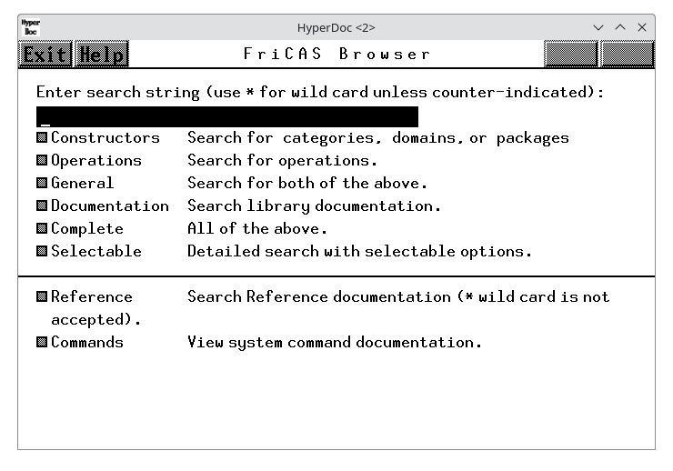
The Browse front page.
To use this page, you first enter a search string into the input area at the top, then click on one of the buttons below. We show the use of each of the buttons by example.
First enter the search string Matrix into the input area and click on Constructors. What you get is the constructor page for Matrix. We show and describe this page in detail in Section 14.2 on page 1531. By convention, FriCAS does a case-insensitive search for a match. Thus matrix is just as good as Matrix, has the same effect as MaTrix, and so on. We recommend that you generally use lowercase letters for names however. A search string with only capital letters has a special meaning (see Section 14.3.3 on page 1570).
Click on to return to the Browse front page.
Use the symbol “*” in search strings as a wildcard.
A wildcard matches any substring, including the empty string. For example, enter the search string *matrix* into the input area and click on Constructors.1 What you get is a table of all constructors whose names contain the string “matrix.”
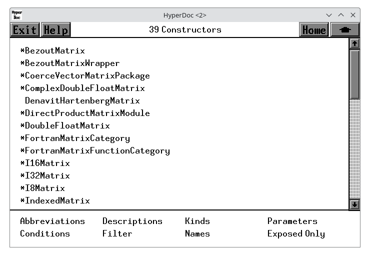
Table of exposed constructors matching *matrix*.
All constructors containing the string are listed, whether exposed or unexposed. You can hide the names of the unexposed constructors by clicking on the *=unexposed button in the Views panel at the bottom of the window. (The button will change to exposed only.)
One of the names in this table is Matrix. Click on Matrix. What you get is again the constructor page for Matrix. As you see, Browse gives you a large network of information in which there are many ways to reach the same pages.
Again click on the to return to the table of constructors whose names contain matrix. Below the table is
a Views panel. This panel contains buttons that let you view constructors in different ways. To learn about
views of constructors, skip to Section 14.2.2 on page 1554.
Click on to return to the Browse front page.
Enter *matrix into the input area and click on Operations. This time you get a table of operations whose names end with matrix or Matrix.
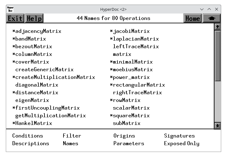
Table of operations matching *matrix.
If you select an operation name, you go to a page describing all the operations in FriCAS of that name. At the bottom of an operation page is another kind of Views panel, one for operation pages. To learn more about these views, skip to Section 14.3.2 on page 1564.
Click on to return to the Browse front page.
This button does a general search for all constructor and operation names matching the search string. Enter the search string *matrix* into the input area. Click on General to find all constructs that have matrix as a part of their name.
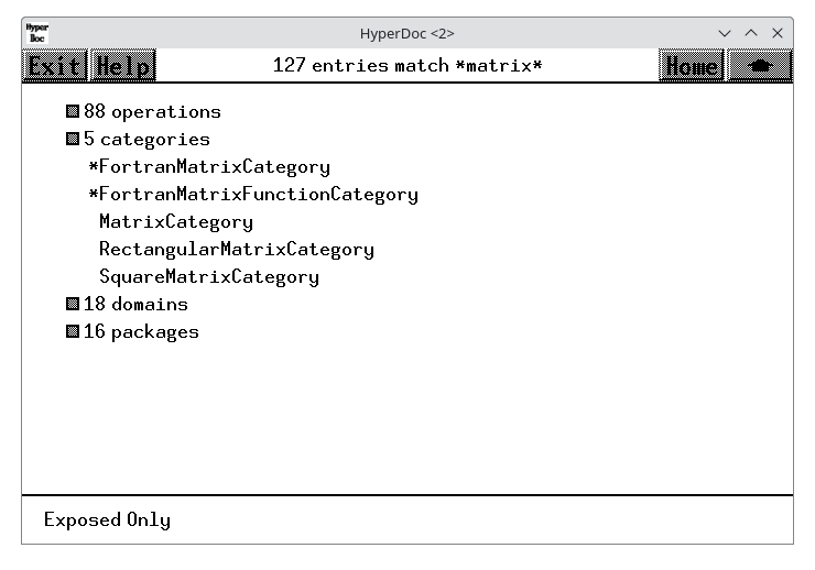
Table of all constructs matching *matrix*.
The summary gives you all the names under a heading when the number of entries is less than 10.
Click on to return to the Browse front page.
Again enter the search key *matrix* and this time click on Documentation. This search matches any constructor and operation name whose documentation contains a substring matching matrix.
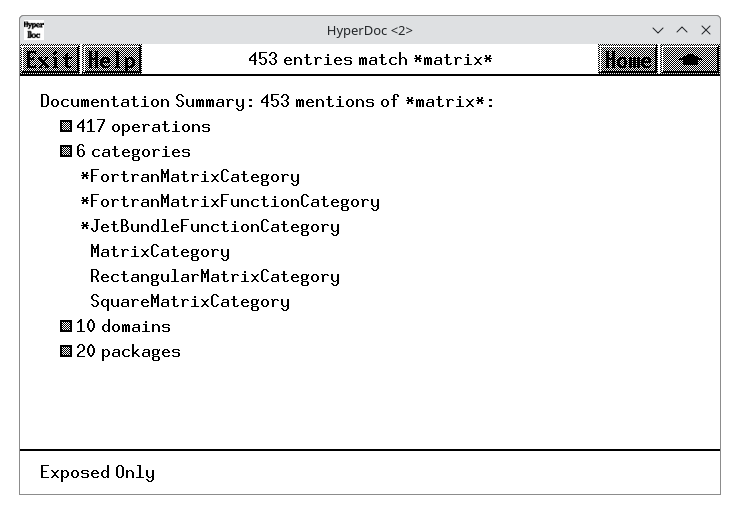
Table of constructs with documentation matching *matrix*.
Click on to return to the Browse front page.
This search combines both General and Documentation.
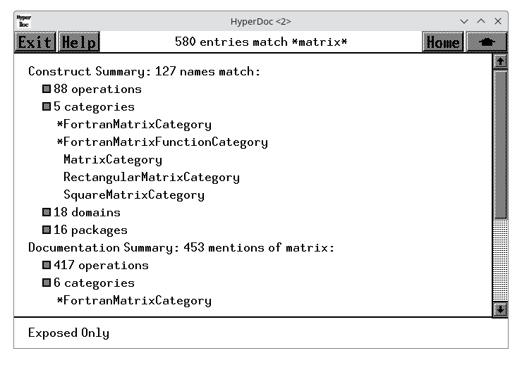
Table summarizing complete search for pattern *matrix*.
In this section we look in detail at a constructor page for domain Matrix. Enter matrix into the input area on the main Browse page and click on Constructors.
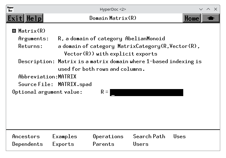
The header part tells you that Matrix takes one argument called R that must be a domain of category AbelianMonoid. Just what domains can be arguments of Matrix? To find this out, click on the R on the second line of the heading. What you get is a table of all acceptable domain parameter values of R, or a table of abelian monoids in FriCAS.
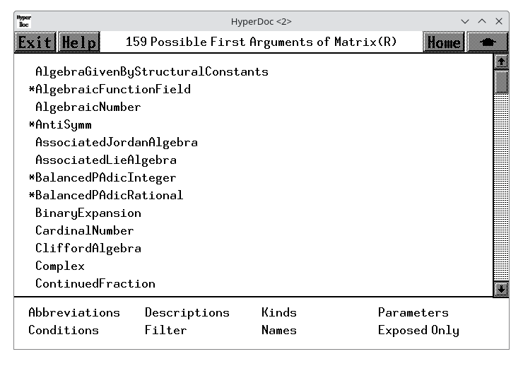
Click on to return to the constructor page for Matrix.
There is also a brief description of constructor Matrix and its abbreviation MATRIX.
If you have access to the source code of FriCAS, this header part also gives you the name of the source file containing the definition of Matrix. Click on it to pop up an editor window containing the source code of Matrix.
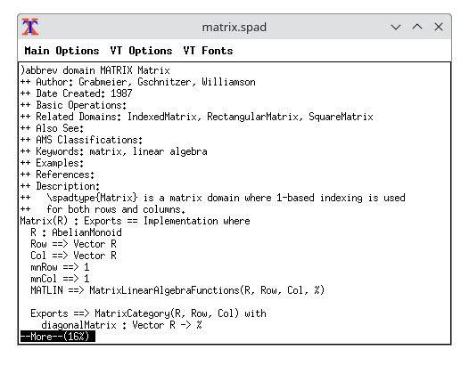
We recommend that you leave the editor window up while working through this chapter as you occasionally may want to refer to it.
We examine each button on this page in order.
Click here to get a table of operations exported by Matrix. You may wish to widen the window to have multiple columns as below.
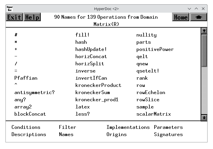
If you click on an operation name, you bring up a description page for the operations. For a detailed description of these pages, skip to Section 14.3.2 on page 1564.
Click here to get an examples page with examples of operations to create and manipulate matrices.
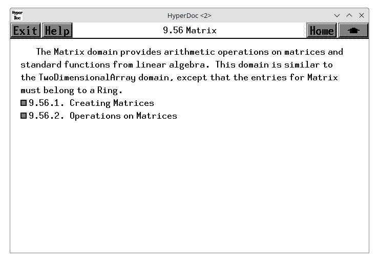
Read through this section. Try selecting the various buttons. Notice that if you click on an operation name, such as new, you bring up a description page for that operation from Matrix.
Example pages have several examples of FriCAS commands. Each example has an active button to its left. Click on it! A pre-computed answer is pasted into the page immediately following the command. If you click on the button a second time, the answer disappears. This button thus acts as a toggle: “now you see it; now you don’t.”
Note also that the FriCAS commands themselves are active. If you want to see FriCAS execute the command, then click on it! A new FriCAS window appears on your screen and the command is executed.
Click here to see a page describing the exports of Matrix exactly as described by the source code.
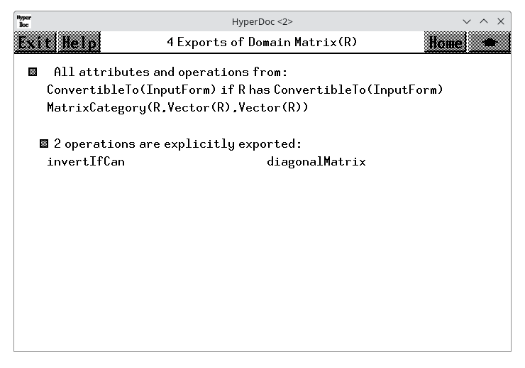
As you see, Matrix declares that it exports all the operations and categories exported by category MatrixCategory(R, Row, Col). In addition, two operations, diagonalMatrix and invertIfCan, are explicitly exported.
To learn a little about the structure of FriCAS, we suggest you do the following exercise. Otherwise, go on to the next section. Matrix explicitly exports only two operations. The other operations are thus exports of MatrixCategory. In general, operations are usually not explicitly exported by a domain. Typically they are inherited from several different categories. Let’s find out from where the operations of Matrix come.
repeatedly to return to the constructor page for Matrix.
The parents of a domain are the same as the categories mentioned under the Exports button on the first page. Domain Matrix has two parents but in general a domain can have any number.
The ancestors of a constructor consist of its parents, the parents of its parents, and so on. Did you perform the exercise in the last section under Exports? If so, you see here all the categories you found while ascending the Exports chain for Matrix.
The dependents of a constructor are those domains or packages that mention that constructor either as an argument or in its exports.
If you click on Dependents two entries may surprise you: RectangularMatrix and SquareMatrix. This happens because Matrix, as it turns out, appears in signatures of operations exported by these domains.
The term search path refers to the search order for functions. If you are an expert user or curious about how the FriCAS system works, try the following exercise. Otherwise, you best skip this button and go on to Users.
Clicking on Search Path gives you a list of domain constructors: InnerIndexedTwoDimensionalArray, MatrixCategory&, TwoDimensionalArrayCategory&, HomogeneousAggregate&, Aggregate&, Evalable&, SetCategory&, Hashable&, InnerEvalable&, BasicType&. What are these constructors and how are they used?
We explain by an example. Suppose you create a matrix using the interpreter, then ask for its rank. FriCAS must then find a function implementing the rank operation for matrices. The first place FriCAS looks for rank is in the Matrix domain.
If not there, the search path of Matrix tells FriCAS where else to look. Associated with the matrix domain are ten other search path domains. Their order is important. FriCAS first searches the first one, InnerIndexedTwoDimensionalArray. If not there, it searches the second MatrixCategory&. And so on.
Where do these search path constructors come from? The source code for Matrix contains this syntax for the function body of Matrix:2
InnerIndexedTwoDimensionalArray(R,mnRow,mnCol,Row,Col) add ...
where the “...” denotes all the code that follows. In English, this means: “The functions for matrices are defined as those from InnerIndexedTwoDimensionalArray domain augmented by those defined in ‘...’,” where the latter take precedence.
This explains InnerIndexedTwoDimensionalArray. The other names, those with names ending with an ampersand “&” are default packages for categories to which Matrix belongs. Default packages are ordered by the notion of “closest ancestor.”
A user of Matrix is any constructor that uses Matrix in its implementation. For example, Complex is a user of Matrix; it exports several operations that take matrices as arguments or return matrices as values.3
A benefactor of Matrix is any constructor that Matrix uses in its implementation. This information, like that for clients, is gathered from run-time structures.4
Cross reference pages for categories have some different buttons on them. Starting with the front page of Browse, search for Ring and enter its constructor page. Here are buttons Parents and Ancestors similar to the notion for domains, except for categories the relationship between parent and child is defined through category extension.
Category hierarchies go both ways. There are children as well as parents.
These are children, children of children, and so on.
Category hierarchies are complicated by the fact that categories take parameters. Where a parameterized category fits into a hierarchy may depend on values of its parameters. In general, the set of categories in FriCAS forms a directed acyclic graph, that is, a graph with directed arcs and no cycles.
This produces a table of all domain constructors that can possibly be rings (members of category Ring). Some domains are unconditional rings. Others are rings for some parameters and not for others. To find out which, select the conditions button in the views panel. For example, DirectProduct(n, R) is a ring if R is a ring.
Below every constructor table page is a Views panel. As an example, click on Uses from the constructor page of Matrix to produce a short table of constructor names.
The Views panel is at the bottom of the page. Two items, names and conditions, are in italics. Others are active buttons. The active buttons are those that give you useful alternative views on this table of constructors. Once you select a view, you notice that the button turns off (becomes italicized) so that you cannot reselect it.
This view gives you a table of names. Selecting any of these names brings up the constructor page for that constructor.
This view gives you a table of abbreviations, in the same order as the original constructor names. Abbreviations are in capitals and they can be used interchangeably with constructor names in input areas.
This view organizes constructor names into the three kinds: categories, domains and packages.
This view presents constructors with the arguments. This view of the benefactors of Matrix shows that Matrix uses as many as ten different List domains in its implementation.
This button is used to refine the list of names or abbreviations. Starting with the names view, enter m* into the input area and click on filter. You then get a shorter table with only the names beginning with m.
This gives you documentation for each of the constructors.
This page organizes the constructors according to predicates. The view is not available for your example page since all constructors are unconditional. For a table with conditions, return to the Ancestors page for Matrix, click on conditions in the view panel. This page shows you that CoercibleTo(OutputForm) and SetCategory are ancestors of Matrix(R) only if R belongs to category SetCategory.
Notice the input area at the bottom of the constructor page. If you leave this blank, then the information you get is for the domain constructor Matrix(R), that is, Matrix for an arbitrary underlying domain R.
In general, however, the exports and other information do usually depend on the actual value of R. For example, Matrix exports the inverse operation only if the domain R is a Field. To see this, try this from the main constructor page:
to return to the constructor page.
Click on inverse to produce a page describing the operation inverse. At the bottom of the description, you notice that the Conditions line says “R has Field.” This operation is not exported by Matrix(Integer) since Integer is not a field.
Try putting the name of a domain such as Fraction Integer (which is a field) into the input area, then clicking on Operations. As you see, the operation inverse is exported.
From the constructor page of Matrix, click on Operations to bring up the table of operations for Matrix.
Find the operation inverse in the table and click on it. This takes you to a page showing the documentation for this operation.
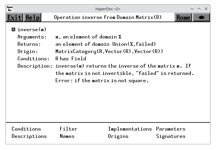
Here is the significance of the headings you see.
This lists each of the arguments of the operation in turn, paraphrasing the signature of the operation. As for signatures, a “%” is used to designate this domain, that is, Matrix(R).
This describes the return value for the operation, analogous to the Arguments part.
This tells you which domain or category explicitly exports the operation. In this example, the Origin is MatrixCategory.
This tells you that the operation is exported by Matrix(R) only if “R has Field,” that is, “R is a member of category Field.” When no Conditions part is given, the operation is exported for all values of R.
Here are the “++” comments that appear in the source code of its Origin, here Matrix. You find these comments in the source code for Matrix.
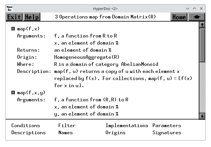
Click on to return to the table of operations. Click on map. Here you find three different operations
named map. This should not surprise you. Operations are identified by name and signature. There are three
operations named map, each with different signatures. What you see is the descriptions view of the
operations. If you like, select the button in the heading of one of these descriptions to get only that
operation.
This part qualifies domain parameters mentioned in the arguments to the operation.
We suggest that you go to the constructor page for Matrix and click on Operations to bring up a table of operations with a Views panel at the bottom.
This view lists the names of the operations. Unlike constructors, however, there may be several operations with the same name. The heading for the page tells you the number of unique names and the number of distinct operations when these numbers are different.
As for constructors, you can use this button to cut down the list of operations you are looking at. Click on filter and enter, for example, m* into the input area, then click on filter. As usual, any logical expression is permitted. For example, use
*! or *?
to get a list of destructive operations and predicates.
This gives you the most information: a detailed description of all the operations in the form you have seen before. Every other button summarizes these operations in some form.
This views the operations by showing their signatures.
This views the operations by their distinct syntactic forms with parameters.
This organizes the operations according to the constructor that explicitly exports them.
This view organizes the operations into conditional and unconditional operations.
This button is only available if your user-level is set to development. The usage button produces a table of constructors that reference this operation.5
This button is only available if your user-level is set to development. If you enter values for all domain parameters on the constructor page, then the implementation button can be clicked. This button tells you what domains or packages actually implement the various operations.6
With your user-level set to development, we suggest you try this exercise. Return to the main constructor page for Matrix, then enter Integer into the input area at the bottom as the value of R. Then click on Operations to produce a table of operations. Click on implementation. After some delay, you get a page describing what implements each of the matrix operations, organized by the various domains and packages.
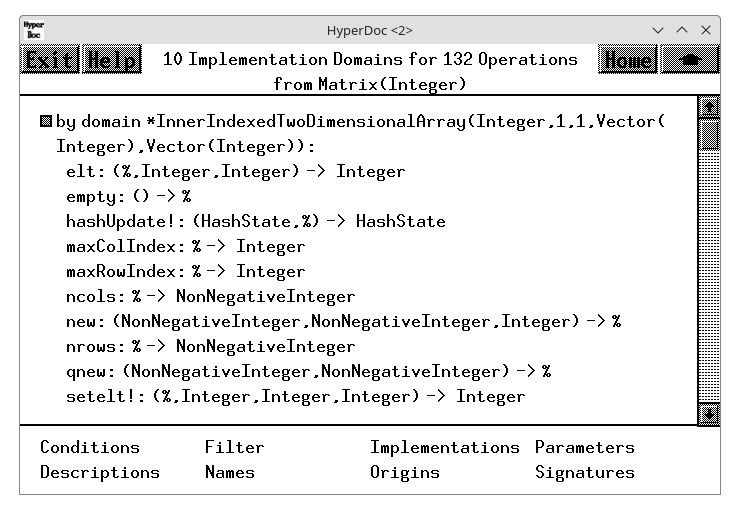
When entering search keys for constructors, you can use capital letters to search for abbreviations. For example, enter UTS into the input area and click on Constructors. Up comes a page describing UnivariateTaylorSeries whose abbreviation is UTS.
Constructor abbreviations always have three or more capital letters. For short constructor names (six letters or less), abbreviations are not generally helpful as their abbreviation is typically the constructor name in capitals. For example, the abbreviation for Matrix is MATRIX.
Abbreviations can also contain numbers. For example, POLY2 is the abbreviation for constructor PolynomialFunctions2. For default packages, the abbreviation is the same as the abbreviation for the corresponding category with the “&” replaced by “-”. For example, for the category default package MatrixCategory& the abbreviation is MATCAT- since the corresponding category MatrixCategory has abbreviation MATCAT.
FriCAS information can be found online at http://fricas.github.io.
Bug fixes, in particular:
Bug fixes, in particular:
Bug fixes, in particular:
Bug fixes, in particular:
Bug fixes, in particular:
Bug fixes, in particular:
Bug fixes, in particular:
Bug fixes, in particular:
Bug fixes, in particular:
Bug fixes, in particular:
Bug fixes, in particular:
Bug fixes, in particular:
Bug fixes, in particular:
Bug fixes, in particular:
Bug fixes, in particular:
Bug fixes, in particular:
Bug fixes, in particular:
Bug fixes, in particular:
error did only minimal checking of its argument. Now argument to error must be a
String or OutputForm or a literal list of OutputForm-s.
Bug fixes, in particular:
%i in patterns.
Bug fixes, in particular:
Bug fixes, in particular:
Bug fixes, in particular:
Bug fixes, in particular:
Bug fixes, in particular:
Bug fixes, in particular:
Bug fixes, in particular:
%.
=> at top level of a function.
**, ^ and 
Bug fixes, in particular:
Bug fixes, in particular:
Bug fixes, in particular:
Bug fixes, in particular:
Bug fixes, in particular:
Bug fixes, in particular:
Bug fixes, in particular:
%e < %pi – now FriCAS will complain about < being undefined.
Bug fixes, in particular:
Several bug fixes, in particular:
The 1.0 release is the first release of FriCAS. Below we list main differences compared to AXIOM September 2006.
Numerous bug fixes (in particular HyperDoc is now fully functional on Unix systems).
FriCAS includes guessing package written by Martin Rubey. This package provides unique ability to guess formulas for sequences of numbers or polynomials.
Some computation, in particular involving Expression domain, should be much faster. FriCAS goes through its testsuite in only half of the time needed by AXIOM September 2006.
Spad compilation is faster (in some cases 2 times faster).
FriCAS is much more portable than AXIOM September 2006. It can be built on Linux, many Unix systems (for example Mac OS X and Solaris 10) and Windows. It can be built on top of gcl, sbcl, clisp or openmcl (gcl and sbcl based FriCAS is fully functional, clisp or openmcl based one lacks graphic support).
Many unused or non-working parts are removed from FriCAS. In particular FriCAS does not contain support for NAG numerical library.
FriCAS can be built from sources using only a few pre-generated Lisp files for bootstrap – only to bootstrap Shoe translator. This means that modifying FriCAS algebra is now much easier.
$ as name of current domain is no longer supported, use % instead.
.01 use 0.01
#1, #2, etc. are no longer supported, to define anonymous functions
use 
{’sin, ’cos}::Set(Symbol) use
set([’sin, ’cos])$Set(Symbol).
:) to denote conversion, like pretend but performing even less checking.
This is no longer supported, use :: or pretend instead.
~=,<=,>,>= in ways which are
correct for linear order, but may conflict with other uses (as partial order or when generating
OutputForm). FriCAS no longer performs this transformation. Similarly, Spad parser no longer
treats ^ and ^= in special way.
import keyword.
**, ^, 

constant keyword).
finally part).
leave construct is removed from FriCAS. Use break instead.
div is no longer a keyword. free, generate, goto are FriCAS keywords.
error did only minimal checking of its argument. Now argument to error must be a String or
OutputForm or a literal list of OutputForm-s.
There are also library changes that affect user code:
** lost its definition as exponentiation, use ^ instead.
^ is no longer used as negation (it means exponentiation now) and ^= no longer means inequality,
use not and ~= instead.
setelt is renamed to setelt!.
has?(op, "even") use
has?(op, ’even)
FriCAS information can be found online at
Many things have changed in this version of AXIOM and we describe many of the more important topics here.
Content removed, NAGLink is no longer included in FriCAS.
The leave keyword has been replaced by the break keyword for compatibility with the new AXIOM
extension language. See section Section 5.4.3 on page 260 for more information.
Curly braces are no longer used to create sets. Instead, use set followed by a bracketed expression. For example,
set [1,2,3,4]
Curly braces are now used to enclose a block (see section Section 5.2 on page 248 for more information). For compatibility, a block can still be enclosed by parentheses as well.
New coercions to and from type Expression have been added. For example, it is now possible to map a polynomial represented as an expression to an appropriate polynomial type.
Various messages have been added or rewritten for clarity.
The FullPartialFractionExpansion domain has been added. This domain computes factor-free full partial fraction expansions. See section ‘FullPartialFractionExpansion’ on page 925 for examples.
We have implemented the Bertrand/Cantor algorithm for integrals of hyperelliptic functions. This brings a major speedup for some classes of algebraic integrals.
We have implemented a new (direct) algorithm for integrating trigonometric functions. This brings a speedup and an improvement in the answer quality.
The SmallFloat domain has been renamed DoubleFloat and SmallInteger has been renamed SingleInteger. The new abbreviations as DFLOAT and SINT, respectively. We have defined the macro SF, the old abbreviation for SmallFloat, to expand to DoubleFloat and modified the documentation and input file examples to use the new names and abbreviations. You should do the same in any private FriCAS files you have.
We have made improvements to the differential equation solvers and there is a new facility for solving systems of first-order linear differential equations. In particular, an important fix was made to the solver for inhomogeneous linear ordinary differential equations that corrected the calculation of particular solutions. We also made improvements to the polynomial and transcendental equation solvers including the ability to solve some classes of systems of transcendental equations.
The efficiency of power series have been improved and left and right expansions of tan(f(x))
at x = a pole of f(x) can now be computed. A number of power series bugs were fixed and the
GeneralUnivariatePowerSeries domain was added. The power series variable can appear in the coefficients
and when this happens, you cannot differentiate or integrate the series. Differentiation and integration with
respect to other variables is supported.
A domain was added for representing asymptotic expansions of a function at an exponential singularity.
For limits, the main new feature is the exponential expansion domain used to treat certain exponential singularities. Previously, such singularities were treated in an ad hoc way and only a few cases were covered. Now AXIOM can do things like
limit( (x+1)^(x+1)/x^x - x^x/(x-1)^(x-1), x = %plusInfinity)
in a systematic way. It only does one level of nesting, though. In other words, if f is a function with a pole, we
can handle exp(f), but not exp(exp(f)).
The computation of integral bases has been improved through careful use of Hermite row reduction. A P-adic algorithm for function fields of algebraic curves in finite characteristic has also been developed.
Miscellaneous: There is improved conversion of definite and indefinite integrals to InputForm; binomial coefficients are displayed in a new way; some new simplifications of radicals have been implemented; the operation complexForm for converting to rectangular coordinates has been added; symmetric product operations have been added to LinearOrdinaryDifferentialOperator.
The buttons on the titlebar and scrollbar have been replaced with ones which have a 3D effect. You can change the foreground and background colors of these “controls” by including and modifying the following lines in your .Xdefaults file.
Axiom.hyperdoc.ControlBackground: White Axiom.hyperdoc.ControlForeground: Black
For various reasons, HyperDoc sometimes displays a secondary window. You can control the size and placement of this window by including and modifying the following line in your .Xdefaults file.
Axiom.hyperdoc.FormGeometry: =950x450+100+0
This setting is a standard X Window System geometry specification: you are requesting a window 950 pixels wide by 450 deep and placed in the upper left corner.
Some key definitions have been changed to conform more closely with the CUA guidelines. Press F9 to see the current definitions.
Input boxes (for example, in the Browser) now accept paste-ins from the X Window System. Use the second button to paste in something you have previously copied or cut. An example of how you can use this is that you can paste the type from a FriCAS computation into the main Browser input box.
We describe here a few additions to the on-line version of the AXIOM book which you can read with HyperDoc.
A section has been added to the graphics chapter, describing how to build two-dimensional graphs from lists of points. An example is given showing how to read the points from a file. See section Section 7.1.9 on page 414 for details.
A further section has been added to that same chapter, describing how to add a two-dimensional graph to a viewport which already contains other graphs. See section Section 7.1.10 on page 430 for details.
Chapter 3 and the on-line HyperDoc help have been unified.
An explanation of operation names ending in “?” and “!” has been added to the first chapter. See the end of the section Section 1.3.6 on page 50 for details.
An expanded explanation of using predicates has been added to the sixth chapter. See the example involving evenRule in the middle of the section Section 6.21 on page 375 for details.
Documentation for the )compile, )library and )load commands has been greatly changed. This reflects the ability of the )compile to now invoke the AXIOM-XL compiler, the impending deletion of the )load command and the new )library command. The )library command replaces )load and is compatible with the compiled output from both the old and new compilers.
Content removed - AXIOM-XL (now using name Aldor) is a separate project.
Univariate polynomial factorization over the integers has been enhanced by updates to the GaloisGroupFactorizer type and friends from Frederic Lehobey (Frederic.Lehobey@lifl.fr, University of Lille I, France).
The package constructor PseudoRemainderSequence provides efficient algorithms by Lionel Ducos (Lionel.Ducos@mathlabo.univ-poitiers.fr, University of Poitiers, France) for computing sub-resultants. This leads to a speed up in many places in FriCAS where sub-resultants are computed (polynomial system solving, algebraic factorization, integration).
Based on this package, the domain constructor NewSparseUnivariatePolynomial extends the constructor SparseUnivariatePolynomial. In a similar way, the NewSparseMultivariatePolynomial extends the constructor SparseUnivariatePolynomial; it also provides some additional operations related to polynomial system solving by means of triangular sets.
Several domain constructors implement regular triangular sets (or regular chains). Among them RegularTriangularSet and SquareFreeRegularTriangularSet. They also implement an algorithm by Marc Moreno Maza (marc@nag.co.uk, NAG) for computing triangular decompositions of polynomial systems. This method is refined in the package LazardSetSolvingPackage in order to produce decompositions by means of Lazard triangular sets. For the case of polynomial systems with finitely many solutions, these decompositions can also be computed by the package LexTriangularPackage.
The domain constructor RealClosure by Renaud Rioboo (Renaud.Rioboo@lip6.fr, University of Paris 6, France) provides the real closure of an ordered field. The implementation is based on interval arithmetic. Moreover, the design of this constructor and its related packages allows an easy use of other codings for real algebraic numbers.
Based on triangular decompositions and the RealClosure constructor, the package ZeroDimensionalSolvePackage provides operations for computing symbolically the real or complex roots of polynomial systems with finitely many solutions.
Polynomial arithmetic with non-commutative variables has been improved too by a contribution of Michel Petitot (Michel.Petitot@lifl.fr, University of Lille I, France). The domain constructors XRecursivePolynomial and XDistributedPolynomial provide recursive and distributed representations for these polynomials. They are the non-commutative equivalents for the SparseMultivariatePolynomial and DistributedMultivariatePolynomial constructors. The constructor LiePolynomial implement Lie polynomials in the Lyndon basis. The constructor XPBWPolynomial manage polynomials with non-commutative variables in the Poincaré-Birkhoff-Witt basis from the Lyndon basis. This allows to compute in the Lie Group associated with a free nilpotent Lie algebra by using the LieExponentials domain constructor.
From this version of AXIOM onwards, the pixmap format used to save graphics images in color and to display them in HyperDoc has been changed to the industry-standard XPM format. See ftp://koala.inria.fr/pub/xpm.
Content removed - NAGLink is no longer included in FriCAS.
Content removed - no longer relevant since FriCAS runs on different Lisp systems.
This chapter describes system commands, the command-line facilities used to control the FriCAS environment. The first section is an introduction and discusses the common syntax of the commands available.
System commands are used to perform FriCAS environment management. Among the commands are those that display what has been defined or computed, set up multiple logical FriCAS environments (frames), clear definitions, read files of expressions and commands, show what functions are available, and terminate FriCAS.
Some commands are restricted: the commands
)set userlevel interpreter )set userlevel compiler )set userlevel development
set the user-access level to the three possible choices. All commands are available at development level and the fewest are available at interpreter level. The default user-level is interpreter. In addition to the )set command (discussed in Section A.20 on page 1705) you can use the HyperDoc settings facility to change the user-level.
Each command listing begins with one or more syntax pattern descriptions plus examples of related commands. The syntax descriptions are intended to be easy to read and do not necessarily represent the most compact way of specifying all possible arguments and options; the descriptions may occasionally be redundant.
All system commands begin with a right parenthesis which should be in the first available column of the input line (that is, immediately after the input prompt, if any). System commands may be issued directly to FriCAS or be included in .input files.
A system command argument is a word that directly follows the command name and is not followed or preceded by a right parenthesis. A system command option follows the system command and is directly preceded by a right parenthesis. Options may have arguments: they directly follow the option. This example may make it easier to remember what is an option and what is an argument:
)syscmd arg1 arg2 )opt1 opt1arg1 opt1arg2 )opt2 opt2arg1 ...
In the system command descriptions, optional arguments and options are enclosed in brackets (“[” and “]”). If an argument or option name is in italics, it is meant to be a variable and must have some actual value substituted for it when the system command call is made. For example, the syntax pattern description
)read fileName [)quietly]
would imply that you must provide an actual file name for fileName but need not use the )quietly option. Thus
)read matrix.input
is a valid instance of the above pattern.
System command names and options may be abbreviated and may be in upper or lower case. The case of actual arguments may be significant, depending on the particular situation (such as in file names). System command names and options may be abbreviated to the minimum number of starting letters so that the name or option is unique. Thus
)s Integer
is not a valid abbreviation for the )set command, because both )set and )show begin with the letter “s”. Typically, two or three letters are sufficient for disambiguating names. In our descriptions of the commands, we have used no abbreviations for either command names or options.
In some syntax descriptions we use a vertical line “|” to indicate that you must specify one of the listed choices. For example, in
)set output fortran on | off
only on and off are acceptable words for following boot. We also sometimes use “...” to indicate that additional arguments or options of the listed form are allowed. Finally, in the syntax descriptions we may also list the syntax of related commands.
User Level Required: compiler
Command Syntax:
)abbreviation query [nameOrAbbrev]
)abbreviation category abbrev fullname [)quiet]
)abbreviation domain abbrev fullname [)quiet]
)abbreviation package abbrev fullname [)quiet]
)abbreviation remove nameOrAbbrev
Command Description:
This command is used to query, set and remove abbreviations for category, domain and package constructors. Every constructor must have a unique abbreviation. This abbreviation is part of the name of the subdirectory under which the components of the compiled constructor are stored. Furthermore, by issuing this command you let the system know what file to load automatically if you use a new constructor. Abbreviations must start with a letter and then be followed by up to seven letters or digits. Any letters appearing in the abbreviation must be in uppercase.
When used with the query argument, this command may be used to list the name associated with a particular abbreviation or the abbreviation for a constructor. If no abbreviation or name is given, the names and corresponding abbreviations for all constructors are listed.
The following shows the abbreviation for the constructor List:
)abbreviation query List
The following shows the constructor name corresponding to the abbreviation NNI:
)abbreviation query NNI
The following lists all constructor names and their abbreviations.
)abbreviation query
To add an abbreviation for a constructor, use this command with category, domain or package. The following add abbreviations to the system for a category, domain and package, respectively:
)abbreviation domain SET Set )abbreviation category COMPCAT ComplexCategory )abbreviation package LIST2MAP ListToMap
If the )quiet option is used, no output is displayed from this command. You would normally only define an abbreviation in a library source file. If this command is issued for a constructor that has already been loaded, the constructor will be reloaded next time it is referenced. In particular, you can use this command to force the automatic reloading of constructors.
To remove an abbreviation, the remove argument is used. This is usually only used to correct a previous command that set an abbreviation for a constructor name. If, in fact, the abbreviation does exist, you are prompted for confirmation of the removal request. Either of the following commands will remove the abbreviation VECTOR2 and the constructor name VectorFunctions2 from the system:
)abbreviation remove VECTOR2 )abbreviation remove VectorFunctions2
Also See: ‘)compile’ in Section A.7 on page 1656 and ‘)library’ in Section A.14 on page 1700.
User Level Required: development
Command Syntax:
)boot bootExpression
Command Description:
This command is used by FriCAS system developers to execute expressions written in the BOOT language. For example,
)boot times3(x) == 3*x
creates and compiles the Common LISP function “times3” obtained by translating the BOOT code.
Also See: ‘)fin’ in Section A.10 on page 1681, ‘)lisp’ in Section A.15 on page 1701, ‘)set’ in Section A.20 on page 1705, and ‘)system’ in Section A.24 on page 1719.
User Level Required: interpreter
Command Syntax:
)cd directory
Command Description:
This command sets the FriCAS working current directory. The current directory is used for looking for input files (for )read), FriCAS library source files (for )compile), saved history environment files (for )history )restore), compiled FriCAS library files (for )library), and files to edit (for )edit). It is also used for writing spool files (via )spool), writing history input files (via )history )write) and history environment files (via )history )save),and compiled FriCAS library files (via )compile).
If issued with no argument, this command sets the FriCAS current directory to your home directory. If an argument is used, it must be a valid directory name. Except for the “)” at the beginning of the command, this has the same syntax as the operating system cd command.
Also See: ‘)compile’ in Section A.7 on page 1656, ‘)edit’ in Section A.9 on page 1678, ‘)history’ in Section A.13 on page 1695, ‘)library’ in Section A.14 on page 1700, ‘)read’ in Section A.19 on page 1704, and ‘)spool’ in Section A.22 on page 1713.
User Level Required: interpreter
Command Syntax:
)close
)close )quietly
Command Description:
This command is used to close down interpreter client processes. Such processes are started by HyperDoc to run FriCAS examples when you click on their text. When you have finished examining or modifying the example and you do not want the extra window around anymore, issue
)close
to the FriCAS prompt in the window.
If you try to close down the last remaining interpreter client process, FriCAS will offer to close down the entire FriCAS session and return you to the operating system by displaying something like
This is the last FriCAS session. Do you want to kill FriCAS?
Type ”y” (followed by the Return key) if this is what you had in mind. Type ”n” (followed by the Return key) to cancel the command.
You can use the )quietly option to force FriCAS to close down the interpreter client process without closing down the entire FriCAS session.
Also See: ‘)quit’ in Section A.18 on page 1703 and ‘)pquit’ in Section A.17 on page 1702.
User Level Required: interpreter
Command Syntax:
)clear all
)clear completely
)clear properties all
)clear properties obj1 [obj2 ...]
)clear value all
)clear value obj1 [obj2 ...]
)clear mode all
)clear mode obj1 [obj2 ...]
Command Description:
This command is used to remove function and variable declarations, definitions and values from the workspace. To empty the entire workspace and reset the step counter to 1, issue
)clear all
To remove everything in the workspace but not reset the step counter, issue
)clear properties all
To remove everything about the object x, issue
)clear properties x
To remove everything about the objects x, y and f, issue
)clear properties x y f
The word properties may be abbreviated to the single letter “p”.
)clear p all )clear p x )clear p x y f
All definitions of functions and values of variables may be removed by either
)clear value all )clear v all
This retains whatever declarations the objects had. To remove definitions and values for the specific objects x, y and f, issue
)clear value x y f )clear v x y f
To remove the declarations of everything while leaving the definitions and values, issue
)clear mode all )clear m all
To remove declarations for the specific objects x, y and f, issue
)clear mode x y f )clear m x y f
The )display names and )display properties commands may be used to see what is currently in the workspace.
The command
)clear completely
does everything that )clear all does, and also clears the internal system function and constructor caches.
Also See: ‘)display’ in Section A.8 on page 1671, ‘)history’ in Section A.13 on page 1695, and ‘)undo’ in Section A.26 on page 1733.
User Level Required: compiler
Command Syntax:
)compile
)compile fileName
)compile fileName.as
)compile directory/fileName.as
)compile fileName.ao
)compile directory/fileName.ao
)compile fileName.al
)compile directory/fileName.al
)compile fileName.lsp
)compile directory/fileName.lsp
)compile fileName.spad
)compile directory/fileName.spad
)compile fileName )new
)compile fileName )old
)compile fileName )quiet
)compile fileName )noquiet
)compile fileName )moreargs
)compile fileName )onlyargs
)compile fileName )break
)compile fileName )nobreak
)compile fileName )library
)compile fileName )nolibrary
)compile fileName )vartrace
)compile fileName )constructor nameOrAbbrev
Command Description:
You use this command to invoke the Aldor library compiler or the FriCAS system compiler. The )compile system command is actually a combination of FriCAS processing and a call to the Aldor compiler. It is performing double-duty, acting as a front-end to both the Aldor compiler and the FriCAS system compiler. (The FriCAS system compiler is written in Boot and is an integral part of the FriCAS environment. The Aldor compiler is written in C and executed by the operating system when called from within FriCAS.)
The command compiles files with file extensions .as, .ao and .al with the Aldor compiler and files with file extension .spad with the FriCAS system compiler. It also can compile files with file extension .lsp. These are assumed to be Lisp files generated by the Aldor compiler. If you omit the file extension, the command looks to see if you have specified the )new or )old option. If you have given one of these options, the corresponding compiler is used. Otherwise, the command first looks in the standard system directories for files with extension .as, .ao and .al and then files with extension .spad. The first file found has the appropriate compiler invoked on it. If the command cannot find a matching file, an error message is displayed and the command terminates.
We now describe the options for the Aldor compiler.
The first thing )compile does is look for a source code filename among its arguments. Thus
)compile mycode.as )compile /u/jones/as/mycode.as )compile mycode
all invoke )compiler on the file /u/jones/as/mycode.as if the current FriCAS working directory is /u/jones/as. (Recall that you can set the working directory via the )cd command. If you don’t set it explicitly, it is the directory from which you started FriCAS.)
This is frequently all you need to compile your file. This simple command:
Should you not want the )library command automatically invoked, call )compile with the )nolibrary option. For example,
)compile mycode.as )nolibrary
The general description of Aldor command line arguments is in the Aldor documentation. The default options used by the )compile command can be viewed and set using the )set compiler args FriCAS system command. The current defaults are
-O -Fasy -Fao -Flsp -lfricas -Mno-ALDOR_W_WillObsolete -DFriCAS -Y $FRICAS/algebra -I $FRICAS/algebra
These options mean:
To supplement these default arguments, use the )moreargs option on )compile. For example,
)compile mycode.as )moreargs "-v"
uses the default arguments and appends the -v (verbose) argument flag. The additional argument specification must be enclosed in double quotes.
To completely replace these default arguments for a particular use of )compile, use the )onlyargs option. For example,
)compile mycode.as )onlyargs "-v -O"
only uses the -v (verbose) and -O (optimize) arguments. The argument specification must be enclosed in double quotes. In this example, Lisp code is not produced and so the compilation output will not be available to FriCAS.
To completely replace the default arguments for all calls to )compile within your FriCAS session, use )set compiler args. For example, to use the above arguments for all compilations, issue
)set compiler args "-v -O"
Make sure you include the necessary -l and -Y arguments along with those needed for Lisp file creation. As above, the argument specification must be enclosed in double quotes.
By default, the )library system command exposes all domains and categories it processes. This means that the FriCAS interpreter will consider those domains and categories when it is trying to resolve a reference to a function. Sometimes domains and categories should not be exposed. For example, a domain may just be used privately by another domain and may not be meant for top-level use. The )library command should still be used, though, so that the code will be loaded on demand. In this case, you should use the )nolibrary option on )compile and the )noexpose option in the )library command. For example,
)compile mycode.as )nolibrary )library mycode )noexpose
Once you have established your own collection of compiled code, you may find it handy to use the )dir option on the )library command. This causes )library to process all compiled code in the specified directory. For example,
)library )dir /u/jones/as/quantum
You must give an explicit directory after )dir, even if you want all compiled code in the current working directory processed, e.g.
)library )dir .
The )compile command works with several file extensions. We saw above what happens when it is invoked on a file with extension .as. A .ao file is a portable binary compiled version of a .as file, and )compile simply passes the .ao file onto Aldor. The generated Lisp file is compiled and )library is automatically called, just as if you had specified a .as file.
A .al file is an archive file containing .ao files. The archive is created (on Unix systems) with the ar program. When )compile is given a .al file, it creates a directory whose name is based on that of the archive. For example, if you issue
)compile mylib.al
the directory mylib.axldir is created. All members of the archive are unarchived into the directory and )compile is called on each .ao file found. It is your responsibility to remove the directory and its contents, if you choose to do so.
A .lsp file is a Lisp source file, presumably, in our context, generated by Aldor when called with the -Flsp option. When )compile is used with a .lsp file, the Lisp file is compiled and )library is called. You must also have present a .asy generated from the same source file.
The following are descriptions of options for the FriCAS system compiler.
You can compile category, domain, and package constructors contained in files with file extension .spad. You can compile individual constructors or every constructor in a file.
The full filename is remembered between invocations of this command and )edit commands. The sequence of commands
)compile matrix.spad )edit )compile
will call the compiler, edit, and then call the compiler again on the file matrix.spad. If you do not specify a directory, the working current directory (see Section A.4 on page 1642) is searched for the file. If the file is not found, the standard system directories are searched.
If you do not give any options, all constructors within a file are compiled. Each constructor should have an )abbreviation command in the file in which it is defined. We suggest that you place the )abbreviation commands at the top of the file in the order in which the constructors are defined. The list of commands serves as a table of contents for the file.
The )library option causes directories containing the compiled code for each constructor to be created in the working current directory. The name of such a directory consists of the constructor abbreviation and the .NRLIB file extension. For example, the directory containing the compiled code for the MATRIX constructor is called MATRIX.NRLIB. The )nolibrary option says that such files should not be created. The default is )library. Note that the semantics of )library and )nolibrary for the Aldor compiler and for the FriCAS system compiler are completely different.
The )vartrace option causes the compiler to generate extra code for the constructor to support conditional tracing of variable assignments. (see Section A.25 on page 1720). Without this option, this code is suppressed and one cannot use the )vars option for the trace command.
The )constructor option is used to specify a particular constructor to compile. All other constructors in the file are ignored. The constructor name or abbreviation follows )constructor. Thus either
)compile matrix.spad )constructor RectangularMatrix
or
)compile matrix.spad )constructor RMATRIX
compiles the RectangularMatrix constructor defined in matrix.spad.
The )break and )nobreak options determine what the FriCASsystem compiler does when it encounters an error. )break is the default and it indicates that processing should stop at the first error. The value of the )set break variable then controls what happens.
Also See: ‘)abbreviation’ in Section A.2 on page 1635, ‘)edit’ in Section A.9 on page 1678, and ‘)library’ in Section A.14 on page 1700.
User Level Required: interpreter
Command Syntax:
)display all
)display properties
)display properties all
)display properties [obj1 [obj2 ...]]
)display value all
)display value [obj1 [obj2 ...]]
)display mode all
)display mode [obj1 [obj2 ...]]
)display names
)display operations opName
Command Description:
This command is used to display the contents of the workspace and signatures of functions with a given name.1
The command
)display names
lists the names of all user-defined objects in the workspace. This is useful if you do not wish to see everything about the objects and need only be reminded of their names.
The commands
)display all )display properties )display properties all
all do the same thing: show the values and types and declared modes of all variables in the workspace. If you have defined functions, their signatures and definitions will also be displayed.
To show all information about a particular variable or user functions, for example, something named d, issue
)display properties d
To just show the value (and the type) of d, issue
)display value d
To just show the declared mode of d, issue
)display mode d
All modemaps for a given operation may be displayed by using )display operations. A modemap is a collection of information about a particular reference to an operation. This includes the types of the arguments and the return value, the location of the implementation and any conditions on the types. The modemap may contain patterns. The following displays the modemaps for the operation complex:
)d op complex
Also See: ‘)clear’ in Section A.6 on page 1645, ‘)history’ in Section A.13 on page 1695, ‘)set’ in Section A.20 on page 1705, ‘)show’ in Section A.21 on page 1711, and ‘)what’ in Section A.27 on page 1736.
User Level Required: interpreter
Command Syntax:
)edit [filename]
Command Description:
This command is used to edit files. It works in conjunction with the )read and )compile commands to remember the name of the file on which you are working. By specifying the name fully, you can edit any file you wish. Thus
)edit /u/julius/matrix.input
will place you in an editor looking at the file /u/julius/matrix.input. By default, the editor is less just for viewing purpose, but if you have a shell environment variable FRICASEDITOR defined, that editor will be used. When FriCAS is running under the X Window System, it will try to open a separate xterm running your editor if it thinks one is necessary. For example, under the Bash shell, if you issue
export FRICASEDITOR=’emacs +$line $name’
then the emacs editor will be used by )edit.
If you do not specify a file name, the last file you edited, read or compiled will be used. If there is no “last file” you will be placed in the editor editing an empty unnamed file.
It is possible to use the )system command to edit a file directly. For example,
)system emacs /etc/rc.tcpip
Also See: ‘)system’ in Section A.24 on page 1719, ‘)compile’ in Section A.7 on page 1656, and ‘)read’ in Section A.19 on page 1704.
User Level Required: development
Command Syntax:
)fin
Command Description:
This command is used by FriCAS developers to leave the FriCAS system and return to the underlying Common LISP system. To return to FriCAS, issue the “(|spad|)” function call to Common LISP.
Also See: ‘)pquit’ in Section A.17 on page 1702 and ‘)quit’ in Section A.18 on page 1703.
User Level Required: interpreter
Command Syntax:
)frame new frameName
)frame drop [frameName]
)frame next
)frame last
)frame names
)frame import frameName [objectName1 [objectName2 ...]]
)set message frame on | off
)set message prompt frame
Command Description:
A frame can be thought of as a logical session within the physical session that you get when you start the system. You can have as many frames as you want, within the limits of your computer’s storage, paging space, and so on. Each frame has its own step number, environment and history. You can have a variable named a in one frame and it will have nothing to do with anything that might be called a in any other frame.
Some frames are created by the HyperDoc program and these can have pretty strange names, since they are generated automatically. To find out the names of all frames, issue
)frame names
It will indicate the name of the current frame.
You create a new frame “quark” by issuing
)frame new quark
The history facility can be turned on by issuing either )set history on or )history )on. If the history facility is on and you are saving history information in a file rather than in the FriCAS environment then a history file with filename quark.axh will be created as you enter commands. If you wish to go back to what you were doing in the “initial” frame, use
)frame next
or
)frame last
to cycle through the ring of available frames to get back to “initial”.
If you want to throw away a frame (say “quark”), issue
)frame drop quark
If you omit the name, the current frame is dropped.
If you do use frames with the history facility on and writing to a file, you may want to delete some of the older history files. These are directories, so you may want to issue a command like rm -r quark.axh to the operating system.
You can bring things from another frame by using )frame import. For example, to bring the f and g from the frame “quark” to the current frame, issue
)frame import quark f g
If you want everything from the frame “quark”, issue
)frame import quark
You will be asked to verify that you really want everything.
There are two )set flags to make it easier to tell where you are.
)set message frame on | off
will print more messages about frames when it is set on. By default, it is off.
)set message prompt frame
will give a prompt that looks like
initial (1) ->
when you start up. In this case, the frame name and step make up the prompt.
Also See: ‘)history’ in Section A.13 on page 1695 and ‘)set’ in Section A.20 on page 1705.
User Level Required: interpreter
Command Syntax:
)help
)help commandName
)help syntax
Command Description:
This command displays help information about system commands. If you issue
)help help
then this very text will be shown. You can also give the name of a system command to display information about it. For example,
)help clear
will display the description of the )clear system command.
The command
)help syntax
will give further information about the FriCAS language syntax.
All this material is available in the FriCAS User Guide and in HyperDoc. In HyperDoc, choose the Commands item from the Reference menu.
User Level Required: interpreter
Command Syntax:
)history )on
)history )off
)history )write historyInputFileName
)history )show [n] [both]
)history )save savedHistoryName
)history )restore [savedHistoryName]
)history )reset
)history )change n
)history )memory
)history )file
%
%%(n)
)set history on | off
Command Description:
The history facility within FriCAS allows you to restore your environment to that of another session and recall previous computational results. Additional commands allow you to review previous input lines and to create an .input file of the lines typed to FriCAS.
FriCAS saves your input and output if the history facility is turned on (which is the default). This information is saved if either of
)set history on )history )on
has been issued. Issuing either
)set history off )history )off
will discontinue the recording of information.
Whether the facility is disabled or not, the value of “%” in FriCAS always refers to the result of the last
computation. If you have not yet entered anything, “%” evaluates to an object of type Variable(’%). The
function “%%” may be used to refer to other previous results if the history facility is enabled. In that case,
%%(n) is the output from step n if n > 0. If n < 0, the step is computed relative to the current step. Thus %%(-1)
is also the previous step, %%(-2), is the step before that, and so on. If an invalid step number is given, FriCAS
will signal an error.
The environment information can either be saved in a file or entirely in memory (the default). Each frame (Section A.11 on page 1681) has its own history database. When it is kept in a file, some of it may also be kept in memory for efficiency. When the information is saved in a file, the name of the file is of the form FRAME.axh where “FRAME” is the name of the current frame. The history file is placed in the current working directory (see Section A.4 on page 1642). Note that these history database files are not text files (in fact, they are directories themselves), and so are not in human-readable format.
The options to the )history command are as follows:
will set the number of steps that are saved in memory to n. This option only has effect when the history data is maintained in a file. If you have issued )history )memory (or not changed the default) there is no need to use )history )change.
will start the recording of information. If the workspace is not empty, you will be asked to confirm this request. If you do so, the workspace will be cleared and history data will begin being saved. You can also turn the facility on by issuing )set history on.
will stop the recording of information. The )history )show command will not work after issuing this command. Note that this command may be issued to save time, as there is some performance penalty paid for saving the environment data. You can also turn the facility off by issuing )set history off.
indicates that history data should be saved in an external file on disk.
indicates that all history data should be kept in memory rather than saved in a file. Note that if you are computing with very large objects it may not be practical to keep this data in memory.
will flush the internal list of the most recent workspace calculations so that the data structures may be garbage collected by the underlying Common LISP system. Like )history )change, this option only has real effect when history data is being saved in a file.
completely clears the environment and restores it to a saved session, if possible. The )save option below allows you to save a session to a file with a given name. If you had issued )history )save jacobi the command )history )restore jacobi would clear the current workspace and load the contents of the named saved session. If no saved session name is specified, the system looks for a file called last.axh.
is used to save a snapshot of the environment in a file. This file is placed in the current working directory (see Section A.4 on page 1642). Use )history )restore to restore the environment to the state preserved in the file. This option also creates an input file containing all the lines of input since you created the workspace frame (for example, by starting your FriCAS session) or last did a )clear all or )clear completely.
can show previous input lines and output results. )show will display up to twenty of the last input lines (fewer if you haven’t typed in twenty lines). )show n will display up to n of the last input lines. )show both will display up to five of the last input lines and output results. )show n both will display up to n of the last input lines and output results.
creates an .input file with the input lines typed since the start of the session/frame or the last )clear all or )clear completely. If historyInputFileName does not contain a period (“.”) in the filename, .input is appended to it. For example, )history )write chaos and )history )write chaos.input both write the input lines to a file called chaos.input in your current working directory. If you issued one or more )undo commands, )history )write eliminates all input lines backtracked over as a result of )undo. You can edit this file and then use )read to have FriCAS process the contents.
Also See: ‘)frame’ in Section A.11 on page 1681, ‘)read’ in Section A.19 on page 1704, ‘)set’ in Section A.20 on page 1705, and ‘)undo’ in Section A.26 on page 1733.
User Level Required: interpreter
Command Syntax:
)library libName1 [libName2 ...]
)library )dir dirName
)library )only objName1 [objlib2 ...]
)library )noexpose
Command Description:
This command replaces the )load system command. The )library command makes available to FriCAS the compiled objects in the libraries listed.
For example, if you )compile dopler.as in your home directory, issue )library dopler to have FriCAS look at the library, determine the category and domain constructors present, update the internal database with various properties of the constructors, and arrange for the constructors to be automatically loaded when needed. If the )noexpose option has not been given, the constructors will be exposed (that is, available) in the current frame.
If you compiled a file with the FriCAS system compiler, you will have an NRLIB present, for example, DOPLER.NRLIB, where DOPLER is a constructor abbreviation. The command )library DOPLER will then do the analysis and database updates as above.
To tell the system about all libraries in a directory, use )library )dir dirName where dirName is an explicit directory. You may specify “.” as the directory, which means the current directory from which you started the system or the one you set via the )cd command. The directory name is required.
You may only want to tell the system about particular constructors within a library. In this case, use the )only option. The command )library dopler )only Test1 will only cause the Test1 constructor to be analyzed, autoloaded, etc..
Finally, each constructor in a library are usually automatically exposed when the )library command is used. Use the )noexpose option if you do not want them exposed. At a later time you can use )set expose add constructor to expose any hidden constructors.
Also See: ‘)cd’ in Section A.4 on page 1642, ‘)compile’ in Section A.7 on page 1656, ‘)frame’ in Section A.11 on page 1681, and ‘)set’ in Section A.20 on page 1705.
User Level Required: development
Command Syntax:
)lisp [lispExpression]
Command Description:
This command is used by FriCAS system developers to have single expressions evaluated by the Common LISP system on which FriCAS is built. The lispExpression is read by the Common LISP reader and evaluated. If this expression is not complete (unbalanced parentheses, say), the reader will wait until a complete expression is entered.
Since this command is only useful for evaluating single expressions, the )fin command may be used to drop out of FriCAS into Common LISP.
Also See: ‘)system’ in Section A.24 on page 1719, ‘)boot’ in Section A.3 on page 1641, and ‘)fin’ in Section A.10 on page 1681.
User Level Required: development
Command Syntax:
This command has the same arguments as options as the )trace command.
Command Description:
This command is used by FriCAS system developers to trace Common LISP or BOOT functions. It is not supported for general use.
Also See: ‘)boot’ in Section A.3 on page 1641, ‘)lisp’ in Section A.15 on page 1701, and ‘)trace’ in Section A.25 on page 1720.
User Level Required: interpreter
Command Syntax:
)pquit
Command Description:
This command is used to terminate FriCAS and return to the operating system. Other than by redoing all your computations or by using the )history )restore command to try to restore your working environment, you cannot return to FriCAS in the same state.
)pquit differs from the )quit in that it always asks for confirmation that you want to terminate FriCAS (the “p” is for “protected”). When you enter the )pquit command, FriCAS responds
Please enter y or yes if you really want to leave the interactive
environment and return to the operating system:
If you respond with y or yes, you will see the message
You are now leaving the FriCAS interactive environment.
Issue the command fricas to the operating system to start a new session.
and FriCAS will terminate and return you to the operating system (or the environment from which you invoked the system). If you responded with something other than y or yes, then the message
You have chosen to remain in the FriCAS interactive environment.
will be displayed and, indeed, FriCAS would still be running.
Also See: ‘)fin’ in Section A.10 on page 1681, ‘)history’ in Section A.13 on page 1695, ‘)close’ in Section A.5 on page 1643, ‘)quit’ in Section A.18 on page 1703, and ‘)system’ in Section A.24 on page 1719.
User Level Required: interpreter
Command Syntax:
)quit
)set quit protected | unprotected
Command Description:
This command is used to terminate FriCAS and return to the operating system. Other than by redoing all your computations or by using the )history )restore command to try to restore your working environment, you cannot return to FriCAS in the same state.
)quit differs from the )pquit in that it asks for confirmation only if the command
)set quit protected
has been issued. Otherwise, )quit will make FriCAS terminate and return you to the operating system (or the environment from which you invoked the system).
The default setting is )set quit unprotected. We suggest that you do not (somehow) assign )quit to be executed when you press, say, a function key.
Also See: ‘)fin’ in Section A.10 on page 1681, ‘)history’ in Section A.13 on page 1695, ‘)close’ in Section A.5 on page 1643, ‘)pquit’ in Section A.17 on page 1702, and ‘)system’ in Section A.24 on page 1719.
User Level Required: interpreter
Command Syntax:
)read [fileName]
)read [fileName] [)quiet] [)ifthere]
Command Description:
This command is used to read .input files into FriCAS. The command
)read matrix.input
will read the contents of the file matrix.input into FriCAS. The “.input” file extension is optional. See Section 4.1 on page 207 for more information about .input files.
This command remembers the previous file you edited, read or compiled. If you do not specify a file name, the previous file will be read.
The )ifthere option checks to see whether the .input file exists. If it does not, the )read command does nothing. If you do not use this option and the file does not exist, you are asked to give the name of an existing .input file.
The )quiet option suppresses output while the file is being read.
At user level “development” the )read command can also handle Boot and Lisp files.
Also See: ‘)compile’ in Section A.7 on page 1656, ‘)edit’ in Section A.9 on page 1678, and ‘)history’ in Section A.13 on page 1695.
User Level Required: interpreter
Command Syntax:
)set
)set label1 [... labelN]
)set label1 [... labelN] newValue
Command Description:
The )set command is used to view or set system variables that control what messages are displayed, the type of output desired, the status of the history facility, the way FriCAS user functions are cached, and so on. Since this collection is very large, we will not discuss them here. Rather, we will show how the facility is used. We urge you to explore the )set options to familiarize yourself with how you can modify your FriCAS working environment. There is a HyperDoc version of this same facility available from the main HyperDoc menu.
The )set command is command-driven with a menu display. It is tree-structured. To see all top-level nodes, issue )set by itself.
)set
Variables with values have them displayed near the right margin. Subtrees of selections have “...” displayed in the value field. For example, there are many kinds of messages, so issue )set message to see the choices.
)set message
The current setting for the variable that displays whether computation times are displayed is visible in the menu displayed by the last command. To see more information, issue
)set message time
This shows that time printing is on now. To turn it off, issue
)set message time off
As noted above, not all settings have so many qualifiers. For example, to change the )quit command to being unprotected (that is, you will not be prompted for verification), you need only issue
)set quit unprotected
Also See: ‘)quit’ in Section A.18 on page 1703.
User Level Required: interpreter
Command Syntax:
)show nameOrAbbrev
)show nameOrAbbrev )operations
Command Description: This command displays information about FriCAS domain, package and category constructors. If no options are given, the )operations option is assumed. For example,
)show POLY )show POLY )operations )show Polynomial )show Polynomial )operations
each display basic information about the Polynomial domain constructor and then provide a listing of operations. Since Polynomial requires a Ring (for example, Integer) as argument, the above commands all refer to an unspecified ring R. In the list of operations, “$” means Polynomial(R).
The basic information displayed includes the signature of the constructor (the name and arguments), the constructor abbreviation, the exposure status of the constructor, and the name of the library source file for the constructor.
If operation information about a specific domain is wanted, the full or abbreviated domain name may be used. For example,
)show POLY INT )show POLY INT )operations )show Polynomial Integer )show Polynomial Integer )operations
are among the combinations that will display the operations exported by the domain Polynomial(Integer) (as opposed to the general domain constructor Polynomial).
Also See: ‘)display’ in Section A.8 on page 1671, ‘)set’ in Section A.20 on page 1705, and ‘)what’ in Section A.27 on page 1736.
User Level Required: interpreter
Command Syntax:
)spool [fileName]
)spool
Command Description:
This command is used to save (spool) all FriCAS input and output into a file, called a spool file. You can only have one spool file active at a time. To start spool, issue this command with a filename. For example,
)spool integrate.out
To stop spooling, issue )spool with no filename.
If the filename is qualified with a directory, then the output will be placed in that directory. If no directory information is given, the spool file will be placed in the current directory. The current directory is the directory from which you started FriCAS or is the directory you specified using the )cd command.
Also See: ‘)cd’ in Section A.4 on page 1642.
User Level Required: interpreter
Command Syntax:
)synonym
)synonym synonym fullCommand
)what synonyms
Command Description:
This command is used to create short synonyms for system command expressions. For example, the following synonyms might simplify commands you often use.
)synonym save history )save )synonym restore history )restore )synonym mail system mail )synonym ls system ls )synonym fortran set output fortran
Once defined, synonyms can be used in place of the longer command expressions. Thus
)fortran on
is the same as the longer
)set fortran output on
To list all defined synonyms, issue either of
)synonym )what synonyms
To list, say, all synonyms that contain the substring “ap”, issue
)what synonyms ap
Also See: ‘)set’ in Section A.20 on page 1705 and ‘)what’ in Section A.27 on page 1736.
User Level Required: interpreter
Command Syntax:
)system cmdExpression
Command Description:
This command may be used to issue commands to the operating system while remaining in FriCAS. The cmdExpression is passed to the operating system for execution.
To get an operating system shell, issue, for example, )system sh. When you enter the key combination, Ctrl–D (pressing and holding the Ctrl key and then pressing the D key) the shell will terminate and you will return to FriCAS. We do not recommend this way of creating a shell because Common LISP may field some interrupts instead of the shell. If possible, use a shell running in another window.
If you execute programs that misbehave you may not be able to return to FriCAS. If this happens, you may have no other choice than to restart FriCAS and restore the environment via )history )restore, if possible.
Also See: ‘)boot’ in Section A.3 on page 1641, ‘)fin’ in Section A.10 on page 1681, ‘)lisp’ in Section A.15 on page 1701, ‘)pquit’ in Section A.17 on page 1702, and ‘)quit’ in Section A.18 on page 1703.
User Level Required: interpreter
Command Syntax:
)trace
)trace )off
)trace function [options]
)trace constructor [options]
)trace domainOrPackage [options]
where options can be one or more of
)after S-expression
)before S-expression
)break after
)break before
)cond S-expression
)count
)count n
)depth n
)local op1 [... opN]
)nonquietly
)nt
)off
)only listOfDataToDisplay
)ops
)ops op1 [... opN ]
)restore
)stats
)stats reset
)timer
)varbreak
)varbreak var1 [... varN ]
)vars
)vars var1 [... varN ]
)within executingFunction
Command Description:
This command is used to trace the execution of functions that make up the FriCAS system, functions defined by users, and functions from the system library. Almost all options are available for each type of function but exceptions will be noted below.
To list all functions, constructors, domains and packages that are traced, simply issue
)trace
To untrace everything that is traced, issue
)trace )off
When a function is traced, the default system action is to display the arguments to the function and the return value when the function is exited. Note that if a function is left via an action such as a THROW, no return value will be displayed. Also, optimization of tail recursion may decrease the number of times a function is actually invoked and so may cause less trace information to be displayed. Other information can be displayed or collected when a function is traced and this is controlled by the various options. Most options will be of interest only to FriCAS system developers. If a domain or package is traced, the default action is to trace all functions exported.
Individual interpreter, lisp or boot functions can be traced by listing their names after )trace. Any options that are present must follow the functions to be traced.
)trace f
traces the function f. To untrace f, issue
)trace f )off
Note that if a function name contains a special character, it will be necessary to escape the character with an underscore
)trace _/D_,1
To trace all domains or packages that are or will be created from a particular constructor, give the constructor name or abbreviation after )trace.
)trace MATRIX )trace List Integer
The first command traces all domains currently instantiated with Matrix. If additional domains are instantiated with this constructor (for example, if you have used Matrix(Integer) and Matrix(Float)), they will be automatically traced. The second command traces List(Integer). It is possible to trace individual functions in a domain or package. See the )ops option below.
The following are the general options for the )trace command.
causes a Common LISP break loop to be entered after exiting the traced function.
causes a Common LISP break loop to be entered before entering the traced function.
is the same as )break before.
causes the system to keep a count of the number of times the traced function is entered. The total can be displayed with )trace )stats and cleared with )trace )stats reset.
causes information about the traced function to be displayed for the first n executions. After the
 execution, the function is untraced.
causes trace information to be shown for only n levels of recursion of the traced function. The command
)trace fib )depth 10
will cause the display of only 10 levels of trace information for the recursive execution of a user function fib.
causes the function arguments and return value to be displayed in the FriCAS monospace two-dimensional math format.
causes the display of additional messages when a function is traced.
This suppresses all normal trace information. This option is useful if the )count or )timer options are used and you are interested in the statistics but not the function calling information.
causes untracing of all or specific functions. Without an argument, all functions, constructors, domains and packages are untraced. Otherwise, the given functions and other objects are untraced. To immediately retrace the untraced functions, issue )trace )restore.
causes only specific trace information to be shown. The items are listed by using the following abbreviations:
display all arguments
display return value
display first argument
display second argument
display the 15th argument, and so on
causes the last untraced functions to be retraced. If additional options are present, they are added to those previously in effect.
causes the display of statistics collected by the use of the )count and )timer options.
resets to 0 the statistics collected by the use of the )count and )timer options.
causes the system to keep a count of execution times for the traced function. The total can be displayed with )trace )stats and cleared with )trace )stats reset.
causes a Common LISP break loop to be entered after the assignment to any of the listed variables in the traced function.
causes the display of the value of any variable after it is assigned in the traced function. Note that library code must have been compiled (see Section A.7 on page 1656) using the )vartrace option in order to support this option.
causes the display of the value of any of the specified variables after they are assigned in the traced function. Note that library code must have been compiled (see Section A.7 on page 1656) using the )vartrace option in order to support this option.
causes the display of trace information only if the traced function is called when the given executingFunction is running.
The following are the options for tracing constructors, domains and packages.
causes local functions of the constructor to be traced. Note that to untrace an individual local function, you must use the fully qualified internal name, using the escape character “_” before the semicolon.
)trace FRAC )local
)trace FRAC_;cancelGcd )off
By default, all operations from a domain or package are traced when the domain or package is traced. This option allows you to specify that only particular operations should be traced. The command
)trace Integer )ops min max _+ _-
traces four operations from the domain Integer. Since + and - are special characters, it is necessary to escape them with an underscore.
Also See: ‘)boot’ in Section A.3 on page 1641, ‘)lisp’ in Section A.15 on page 1701, and ‘)ltrace’ in Section A.16 on page 1701.
User Level Required: interpreter
Command Syntax:
)undo
)undo integer
)undo integer [option]
)undo )redo
where option is one of
)after
)before
Command Description:
This command is used to restore the state of the user environment to an earlier point in the interactive session. The argument of an )undo is an integer which must designate some step number in the interactive session.
)undo n )undo n )after
These commands return the state of the interactive environment to that immediately after step n. If n is a
positive number, then n refers to step number n. If n is a negative number, it refers to the  previous
command (that is, undoes the effects of the last
 commands).
A )clear all resets the )undo facility. Otherwise, an )undo undoes the effect of )clear with options
properties, value, and mode, and that of a previous undo. If any such system commands are given between
steps  and
 (
 ), their effect is undone for )undo m for any
 .
The command )undo is equivalent to )undo -1 (it undoes the effect of the previous user expression). The command )undo 0 undoes any of the above system commands issued since the last user expression.
)undo n )before
This command returns the state of the interactive environment to that immediately before step n. Any )undo or )clear system commands given before step n will not be undone.
)undo )redo
This command reads the file redo.input. created by the last )undo command. This file consists of all user input lines, excluding those backtracked over due to a previous )undo.
The command )history )write will eliminate the “undone” command lines of your program.
Also See: ‘)history’ in Section A.13 on page 1695.
User Level Required: interpreter
Command Syntax:
)what categories pattern1 [pattern2 ...]
)what commands pattern1 [pattern2 ...]
)what domains pattern1 [pattern2 ...]
)what operations pattern1 [pattern2 ...]
)what packages pattern1 [pattern2 ...]
)what synonym pattern1 [pattern2 ...]
)what things pattern1 [pattern2 ...]
)apropos pattern1 [pattern2 ...]
Command Description:
This command is used to display lists of things in the system. The patterns are all strings and, if present, restrict the contents of the lists. Only those items that contain one or more of the strings as substrings are displayed. For example,
)what synonym
displays all command synonyms,
)what synonym ver
displays all command synonyms containing the substring “ver”,
)what synonym ver pr
displays all command synonyms containing the substring “ver” or the substring “pr”. Output similar to the following will be displayed
---------------- System Command Synonyms ----------------- user-defined synonyms satisfying patterns: ver pr )apr ........................... )what things )apropos ....................... )what things )prompt ........................ )set message prompt )version ....................... )lisp *yearweek*
Several other things can be listed with the )what command:
displays a list of system commands available at your user-level. Your user-level is set via the )set userlevel command. To get a description of a particular command, such as “)what”, issue )help what.
displays a list of operations in the system library. It is recommended that you qualify this command with one or more patterns, as there are thousands of operations available. For example, say you are looking for functions that involve computation of eigenvalues. To find their names, try )what operations eig. A rather large list of operations is loaded into the workspace when this command is first issued. This list will be deleted when you clear the workspace via )clear all or )clear completely. It will be re-created if it is needed again.
displays all of the above types for items containing the pattern strings as substrings. The command synonym )apropos is equivalent to )what things.
Also See: ‘)display’ in Section A.8 on page 1671, ‘)set’ in Section A.20 on page 1705, and ‘)show’ in Section A.21 on page 1711.
This appendix contains the FriCAS programs used to generate the images in the FriCAS Images color insert of this book. All these input files are included with the FriCAS system. To produce the images on page 6 of the FriCAS Images insert, for example, issue the command:
)read images6
These images were produced on an IBM RS/6000 model 530 with a standard color graphics adapter. The smooth shaded images were made from X Window System screen dumps. The remaining images were produced with FriCAS-generated PostScript output. The images were reproduced from slides made on an Agfa ChromaScript PostScript interpreter with a Matrix Instruments QCR camera.
1)read tknot -- Readtorusknotprogram. 2 3torusKnot(15,17, 0.1, 6, 700) --A(15,17)torus knot. 4
These images illustrate how Newton’s method converges when computing the complex cube roots of 2. Each
point in the  -plane represents the complex number
 which is given as a starting point for
Newton’s method. The poles in these images represent bad starting values. The flat areas are the regions of
convergence to the three roots.
1)read newton --Readtheprograms from 2)read vectors --Chapter 10. 3f := newtonStep(x^3 - 2) --CreateaNewton’s iteration 4 --functionfor. 5
The function  computes
 steps of Newton’s method.
6clipValue := 4 -- Clipvalueswithmagnitude. 7drawComplexVectorField(f^3, -3..3, -3..3) --The vectorfieldfor
8drawComplex(f^3, -3..3, -3..3) --Thesurfacefor
9drawComplex(f^4, -3..3, -3..3) --Thesurfacefor
10
1)r tknot 2for i in 0..4 repeat torusKnot(2, 2 + i/4, 0.5, 25, 250) 3
The parameterization of the Etruscan Venus is due to George Frances.
1venus(a,r,steps) == 2 surf := (u:DFLOAT, v:DFLOAT): Point DFLOAT +-> 3 cv := cos(v) 4 sv := sin(v) 5 cu := cos(u) 6 su := sin(u) 7 x := r * cos(2*u) * cv + sv * cu 8 y := r * sin(2*u) * cv - sv * su 9 z := a * cv 10 point [x,y,z] 11 draw(surf, 0..%pi, -%pi..%pi, var1Steps==steps, 12 var2Steps==steps, title == "Etruscan Venus") 13 14venus(5/2, 13/10, 50) -- TheEtruscanVenus 15
The Figure-8 Klein Bottle parameterization is from “Differential Geometry and Computer Graphics” by Thomas Banchoff, in Perspectives in Mathematics, Anniversary of Oberwolfach 1984, Birkhäuser-Verlag, Basel, pp. 43-60.
16klein(x,y) == 17 cx := cos(x) 18 cy := cos(y) 19 sx := sin(x) 20 sy := sin(y) 21 sx2 := sin(x/2) 22 cx2 := cos(x/2) 23 sq2 := sqrt(2.0@DFLOAT) 24 point [cx * (cx2 * (sq2 + cy) + (sx2 * sy * cy)), _ 25 sx * (cx2 * (sq2 + cy) + (sx2 * sy * cy)), _ 26 -sx2 * (sq2 + cy) + cx2 * sy * cy] 27 28draw(klein, 0..4*%pi, 0..2*%pi, var1Steps==50, -- Figure-8Kleinbottle 29 var2Steps==50,title=="Figure Eight Klein Bottle") 30
The next two images are examples of generalized tubes.
31)read ntube 32rotateBy(p, theta) == --Rotateapointby 33 c := cos(theta) --
aroundtheorigin. 34 s := sin(theta) 35 point [p.1*c - p.2*s, p.1*s + p.2*c] 36 37bcircle t == -- Acircleinthree-space. 38 point [3*cos t, 3*sin t, 0] 39 40twist(u, t) == -- Anellipsethattwists 41 theta := 4*t --aroundfourtimesas 42 p := point [sin u, cos(u)/2] -- trevolvesonce. 43 rotateBy(p, theta) 44 45ntubeDrawOpt(bcircle, twist, 0..2*%pi, 0..2*%pi, -- TwistedTorus 46 var1Steps == 70, var2Steps == 250) 47 48twist2(u, t) == -- Createatwistingcircle. 49 theta := t 50 p := point [sin u, cos(u)] 51 rotateBy(p, theta) 52 53cf(u,v) == sin(21*u) -- Colorfunctionwith21stripes. 54 55ntubeDrawOpt(bcircle, twist2, 0..2*%pi, 0..2*%pi, --Striped Torus 56 colorFunction == cf, var1Steps == 168, 57 var2Steps == 126) 58
1gam(x,y) == --Theheightandcolorarethe 2 g := Gamma complex(x,y) -- realandargumentparts 3 point [x,y,max(min(real g, 4), -4), argument g] --oftheGamma function, 4 --respectively. 5 6draw(gam, -%pi..%pi, -%pi..%pi, -- TheGammaFunction 7 title == "Gamma(x + %i*y)", _ 8 var1Steps == 100, var2Steps == 100) 9 10b(x,y) == Beta(x,y) 11 12draw(b, -3.1..3, -3.1 .. 3, title == "Beta(x,y)") -- TheBetaFunction 13 14atf(x,y) == 15 a := atan complex(x,y) 16 point [x,y,real a, argument a] 17 18draw(atf, -3.0..%pi, -3.0..%pi) -- TheArctangentfunction 19
First we look at the conformal map  .
1)read conformal --Readprogramfor drawing 2 --conformal maps. 3 4f z == z --Thecoordinategridfor the 5 --complex plane. 6conformalDraw(f, -2..2, -2..2, 9, 9, "cartesian") --Mapping1: Source 7 8f z == z + 1/z --Themap9 10conformalDraw(f, -2..2, -2..2, 9, 9, "cartesian") --Mapping1:Target 11
The map  maps the unit disk to the right half-plane, as shown on the Riemann
sphere.
12f z == z --Theunit disk. 13 14riemannConformalDraw(f,0.1..0.99,0..2*%pi,7,11,"polar") --Mapping2: Source 15 16f z == -(z+1)/(z-1) --Themap. 17riemannConformalDraw(f,0.1..0.99,0..2*%pi,7,11,"polar") --Mapping2: Target 18 19riemannSphereDraw(-4..4, -4..4, 7, 7, "cartesian") --RiemannSphereMapping 20
1)read dhtri 2)read tetra 3drawPyramid 4 --Sierpinsky’sTetrahedron 4 5\index{Sierpinsky’s Tetrahedron} 6)read antoine 7drawRings 2 -- Antoine’sNecklace 8 9\index{Antoine’s Necklace} 10)read scherk 11drawScherk(3,3) -- Scherk’sMinimalSurface 12 13\index{Scherk’s minimal surface} 14)read ribbonsNew 15drawRibbons([x^i for i in 1..5], x=-1..1, y=0..2) -- RibbonPlot 16
The functions in this section draw conformal maps both on the plane and on the Riemann sphere.
1C := Complex DoubleFloat --Complex Numbers 2S := Segment DoubleFloat --Draw ranges 3R3 := Point DFLOAT --Pointsin3-space 6
conformalDraw(f, rRange, tRange, rSteps, tSteps, coord) draws the image of the coordinate grid
under f in the complex plane. The grid may be given in either polar or Cartesian coordinates.
Argument f is the function to draw; rRange is the range of the radius (in polar) or real (in Cartesian);
tRange is the range of  (in polar) or imaginary (in Cartesian); tSteps, rSteps, are the number of
intervals in the r and
 directions; and coord is the coordinate system to use (either "polar" or
"cartesian").
7conformalDraw: (C -> C, S, S, PI, PI, String) -> VIEW3D 8conformalDraw(f,rRange,tRange,rSteps,tSteps,coord) == 9 transformC := -- Functionforchangingan10 coord = "polar" => polar2Complex --pairinto acomplexnumber. 11 cartesian2Complex 12 cm := makeConformalMap(f, transformC) 13 sp := createThreeSpace() -- Createafreshspace. 14 adaptGrid(sp, cm, rRange, tRange, rSteps, tSteps) --Plotthecoordinate lines. 15 makeViewport3D(sp, "Conformal Map") --Drawtheimage. 16
riemannConformalDraw(f, rRange, tRange, rSteps, tSteps, coord) draws the image of the coordinate grid under f on the Riemann sphere. The grid may be given in either polar or Cartesian coordinates. Its arguments are the same as those for conformalDraw.
17riemannConformalDraw:(C->C,S,S,PI,PI,String)->VIEW3D 18riemannConformalDraw(f, rRange, tRange, 19 rSteps, tSteps, coord) == 20 transformC := -- Functionforchangingan21 coord = "polar" => polar2Complex --pairinto acomplexnumber. 22 cartesian2Complex 23 sp := createThreeSpace() -- Createafreshspace. 24 cm := makeRiemannConformalMap(f, transformC) 25 adaptGrid(sp, cm, rRange, tRange, rSteps, tSteps) -- Plotthecoordinatelines. 26 curve(sp,[point [0,0,2.0@DFLOAT,0],point [0,0,2.0@DFLOAT,0]]) --Add aninvisiblepointat 27 makeViewport3D(sp,"Map on the Riemann Sphere") --thenorthpolefor scaling. 28 29adaptGrid(sp, f, uRange, vRange, uSteps, vSteps) == --Plotthecoordinategrid 30 delU := (high(uRange) - low(uRange))/uSteps -- usingadaptiveplottingfor 31 delV := (high(vRange) - low(vRange))/vSteps --coordinate lines,anddraw 32 uSteps := uSteps + 1; vSteps := vSteps + 1 --tubesaroundthelines. 33 u := low uRange 34 for i in 1..uSteps repeat -- Drawcoordinatelinesinthev 35 c := curryLeft(f,u) --direction;curve cfixesthe 36 cf := (t:DFLOAT):DFLOAT +-> 0 --currentvalueofu. 37 makeObject(c,vRange::SEG Float,colorFunction==cf, -- Drawthevcoordinateline. 38 space == sp, tubeRadius == .02, tubePoints == 6) 39 u := u + delU 40 v := low vRange 41 for i in 1..vSteps repeat -- Drawcoordinatelinesintheu 42 c := curryRight(f,v) --direction;curve cfixesthe 43 cf := (t:DFLOAT):DFLOAT +-> 1 --currentvalueofv. 44 makeObject(c,uRange::SEG Float,colorFunction==cf, -- Drawtheucoordinateline. 45 space == sp, tubeRadius == .02, tubePoints == 6) 46 v := v + delV 47 void() 48 49riemannTransform(z) == -- Mapapointinthecomplex 50 r := sqrt norm z --planetotheRiemann sphere. 51 cosTheta := (real z)/r 52 sinTheta := (imag z)/r 53 cp := 4*r/(4+r^2) 54 sp := sqrt(1-cp*cp) 55 if r>2 then sp := -sp 56 point [cosTheta*cp, sinTheta*cp, -sp + 1] 57 58cartesian2Complex(r:DFLOAT, i:DFLOAT):C == -- ConvertCartesiancoordinatesto 59 complex(r, i) --complexCartesian form. 60 61polar2Complex(r:DFLOAT, th:DFLOAT):C == --Convertpolarcoordinatesto 62 complex(r*cos(th), r*sin(th)) -- complexCartesianform. 63 64makeConformalMap(f, transformC) == --Convertcomplex functionftoa 65 (u:DFLOAT,v:DFLOAT):R3 +-> --mapping:(DFLOAT,DFLOAT)
R3 66 z := f transformC(u, v) --inthecomplexplane. 67 point [real z, imag z, 0.0@DFLOAT] 68 69makeRiemannConformalMap(f, transformC) == -- Convertacomplexfunctionftoa 70 (u:DFLOAT, v:DFLOAT):R3 +-> --mapping: (DFLOAT,DFLOAT)
R3 71 riemannTransform f transformC(u, v) --onthe Riemannsphere. 72 73riemannSphereDraw: (S, S, PI, PI, String) -> VIEW3D --Drawapictureofthe mapping 74riemannSphereDraw(rRange,tRange,rSteps,tSteps,coord) == --ofthecomplexplaneto 75 transformC := -- theRiemannsphere. 76 coord = "polar" => polar2Complex 77 cartesian2Complex 78 grid := (u:DFLOAT, v:DFLOAT): R3 +-> -- Coordinategridfunction. 79 z1 := transformC(u, v) 80 point [real z1, imag z1, 0] 81 sp := createThreeSpace() -- Createafreshspace. 82 adaptGrid(sp, grid, rRange, tRange, rSteps, tSteps) --Drawtheflatgrid. 83 connectingLines(sp,grid,rRange,tRange,rSteps,tSteps) 84 makeObject(riemannSphere,0..2*%pi,0..%pi,space==sp) -- Drawthesphere. 85 f := (z:C):C +-> z 86 cm := makeRiemannConformalMap(f, transformC) 87 adaptGrid(sp, cm, rRange, tRange, rSteps, tSteps) -- Drawthespheregrid. 88 makeViewport3D(sp, "Riemann Sphere") 89 90connectingLines(sp,f,uRange,vRange,uSteps,vSteps) == -- Drawthelinesthatconnect 91 delU := (high(uRange) - low(uRange))/uSteps --thepoints inthecomplex 92 delV := (high(vRange) - low(vRange))/vSteps --planetothenorthpole 93 uSteps := uSteps + 1; vSteps := vSteps + 1 -- oftheRiemannsphere. 94 u := low uRange 95 for i in 1..uSteps repeat -- Foreachu. 96 v := low vRange 97 for j in 1..vSteps repeat --Foreach v. 98 p1 := f(u,v) 99 p2 := riemannTransform complex(p1.1, p1.2) --Projectp1onto thesphere. 100 fun := lineFromTo(p1,p2) --Createalinefunction. 101 cf := (t:DFLOAT):DFLOAT +-> 3 102 makeObject(fun, 0..1,space==sp,tubePoints==4, -- Drawtheconnectingline. 103 tubeRadius==0.01,colorFunction==cf) 104 v := v + delV 105 u := u + delU 106 void() 107 108riemannSphere(u,v) == -- Aspheresittingonthe 109 sv := sin(v) --complexplane,with radius1. 110 0.99@DFLOAT*(point [cos(u)*sv,sin(u)*sv,cos(v),0.0@DFLOAT])+ 111 point [0.0@DFLOAT, 0.0@DFLOAT, 1.0@DFLOAT, 4.0@DFLOAT] 112 113lineFromTo(p1, p2) == -- Createalinefunction 114 d := p2 - p1 --thatgoesfromp1to p2 115 (t:DFLOAT):Point DFLOAT +-> 116 p1 + t*d 117
Create a  torus-knot with radius
 around the curve. The formula was derived by Larry
Lambe.
1)read ntube 2torusKnot: (DFLOAT, DFLOAT, DFLOAT, PI, PI) -> VIEW3D 3torusKnot(p, q ,r, uSteps, tSteps) == 4 knot := (t:DFLOAT):Point DFLOAT +-> -- Functionforthetorusknot. 5 fac := 4/(2.2@DFLOAT-sin(q*t)) 6 fac * point [cos(p*t), sin(p*t), cos(q*t)] 7 circle := (u:DFLOAT, t:DFLOAT): Point DFLOAT +-> -- Thecrosssection. 8 r * point [cos u, sin u] 9 ntubeDrawOpt(knot, circle, 0..2*%pi, 0..2*%pi, -- Drawthecirclearoundtheknot. 10 var1Steps == uSteps, var2Steps == tSteps) 13
The functions in this file create generalized tubes (also known as generalized cylinders). These functions draw a 2-d curve in the normal planes around a 3-d curve.
1R3 := Point DFLOAT --Pointsin 3-Space 2R2 := Point DFLOAT --Pointsin 2-Space 3S := Segment Float --Draw ranges 4 --Introduce typesforfunctionsfor: 5ThreeCurve := DFLOAT -> R3 --—thespacecurve function 6TwoCurve := (DFLOAT, DFLOAT) -> R2 -- —theplanecurvefunction 7Surface := (DFLOAT, DFLOAT) -> R3 --—thesurface function 8 --Frenet framesdefinea 9FrenetFrame := --coordinatesystemaround a 10 Record(value:R3,tangent:R3,normal:R3,binormal:R3) -- pointonaspacecurve. 11frame: FrenetFrame --ThecurrentFrenet frame 12 --forapointonacurve. 13
ntubeDraw(spaceCurve, planeCurve, 
 draws planeCurve in the normal planes of spaceCurve.
The parameter
 specifies the parameter range for planeCurve and
 specifies the parameter range
for spaceCurve. Additionally, the plane curve function takes a second parameter: the current parameter of
spaceCurve. This allows the plane curve to change shape as it goes around the space curve. See Section B.4 on
page 1745 for an example of this.
14ntubeDraw: (ThreeCurve,TwoCurve,S,S) -> VIEW3D 15ntubeDraw(spaceCurve,planeCurve,uRange,tRange) == 16 ntubeDrawOpt(spaceCurve, planeCurve, uRange, _ 17 tRange, []$List DROPT) 18 19ntubeDrawOpt: (ThreeCurve,TwoCurve,S,S,List DROPT) 20 -> VIEW3D 21ntubeDrawOpt(spaceCurve,planeCurve,uRange,tRange,l) == -- Thisfunctionissimilar 22 --tontubeDraw,buttakes 23 delT:DFLOAT := (high(tRange) - low(tRange))/10000 -- optionalparametersthatit 24 oldT:DFLOAT := low(tRange) - 1 --passestothe drawcommand. 25 fun := ngeneralTube(spaceCurve,planeCurve,delT,oldT) 26 draw(fun, uRange, tRange, l) 29
nfrenetFrame(c, t, delT) numerically computes the Frenet frame about the curve c at t. Parameter delT is a small number used to compute derivatives.
30nfrenetFrame(c, t, delT) == 31 f0 := c(t) 32 f1 := c(t+delT) 33 t0 := f1 - f0 -- Thetangent. 34 n0 := f1 + f0 35 b := cross(t0, n0) --Thebinormal. 36 n := cross(b,t0) -- Thenormal. 37 ln := length n 38 lb := length b 39 ln = 0 or lb = 0 => 40 error "Frenet Frame not well defined" 41 n := (1/ln)*n -- Makeintounitlengthvectors. 42 b := (1/lb)*b 43 [f0, t0, n, b]$FrenetFrame 44
ngeneralTube(spaceCurve, planeCurve,delT, oltT) creates a function that can be passed to the system draw command. The function is a parameterized surface for the general tube around spaceCurve. delT is a small number used to compute derivatives. oldT is used to hold the current value of the t parameter for spaceCurve. This is an efficiency measure to ensure that frames are only computed once for each value of t.
45ngeneralTube: (ThreeCurve, TwoCurve, DFLOAT, DFLOAT) -> Surface 46ngeneralTube(spaceCurve, planeCurve, delT, oldT) == 47 free frame -- Indicatethatframeisglobal. 48 (v:DFLOAT, t: DFLOAT): R3 +-> 49 if (t ~= oldT) then -- Ifnotalreadycomputed, 50 frame := nfrenetFrame(spaceCurve, t, delT) --computenew frame. 51 oldT := t 52 p := planeCurve(v, t) 53 frame.value + p.1*frame.normal + p.2*frame.binormal -- Projectpintothenormalplane. 54
Create affine transformations (DH matrices) that transform a given triangle into another.
1tri2tri: (List Point DFLOAT, List Point DFLOAT) -> DHMATRIX(DFLOAT) 2 -- ComputeaDHMATRIXthat 3tri2tri(t1, t2) == --transformst1 tot2,where 4 n1 := triangleNormal(t1) --t1andt2arethevertices 5 n2 := triangleNormal(t2) -- oftwotrianglesin3-space. 6 tet2tet(concat(t1, n1), concat(t2, n2)) 7 8tet2tet: (List Point DFLOAT, List Point DFLOAT) -> DHMATRIX(DFLOAT) 9 -- ComputeaDHMATRIXthat 10tet2tet(t1, t2) == --transformst1 tot2, 11 m1 := makeColumnMatrix t1 --wheret1andt2arethe 12 m2 := makeColumnMatrix t2 -- verticesoftwotetrahedrons 13 m2 * inverse(m1) --in3-space. 14 15makeColumnMatrix(t) == -- Puttheverticesofatetra- 16 m := new(4,4,0)$DHMATRIX(DFLOAT) --hedroninto matrixform. 17 for x in t for i in 1..repeat 18 for j in 1..3 repeat 19 m(j,i) := x.j 20 m(4,i) := 1 21 m 22 23triangleNormal(t) == -- Computeavectornormalto 24 a := triangleArea t --thegiventriangle, whose 25 p1 := t.2 - t.1 --lengthisthesquareroot 26 p2 := t.3 - t.2 -- oftheareaofthetriangle. 27 c := cross(p1, p2) 28 len := length(c) 29 len = 0 => error "degenerate triangle!" 30 c := (1/len)*c 31 t.1 + sqrt(a) * c 32 33triangleArea t == -- Computetheareaofa 34 a := length(t.2 - t.1) --triangleusingHeron’s 35 b := length(t.3 - t.2) -- formula. 36 c := length(t.1 - t.3) 37 s := (a+b+c)/2 38 sqrt(s*(s-a)*(s-b)*(s-c)) 39
1)set expose add con DenavitHartenbergMatrix --BringDHmatricesintothe 2 -- environment. 3x1:DFLOAT := sqrt(2.0@DFLOAT/3.0@DFLOAT) --Setupthecoordinatesofthe 4x2:DFLOAT := sqrt(3.0@DFLOAT)/6 -- cornersofthetetrahedron. 5 6z := 0.0@DFLOAT 7h := 0.5@DFLOAT 8 9p1 := point [-h, -x2, z] -- Someneededpoints. 10p2 := point [h, -x2, z] 11p3 := point [z, 2*x2, z] 12p4 := point [z, z, x1] 13 14baseTriangle := [p2, p1, p3] -- Thebaseofthetetrahedron. 15 16mt := [h*(p2+p1), h*(p1+p3), h*(p3+p2)] --The“middle triangle”inscribed 17 --inthebaseofthetetrahedron. 18bt1 := [mt.1, p1, mt.2] -- Thebasesofthetrianglesof 19bt2 := [p2, mt.1, mt.3] --thesubdivided tetrahedron. 20bt3 := [mt.2, p3, mt.3] 21bt4 := [h*(p2+p4), h*(p1+p4), h*(p3+p4)] 22 23tt1 := tri2tri(baseTriangle, bt1) -- Createthetransformations 24tt2 := tri2tri(baseTriangle, bt2) --thatbringthe baseofthe 25tt3 := tri2tri(baseTriangle, bt3) --tetrahedrontothebasesof 26tt4 := tri2tri(baseTriangle, bt4) -- thesubdividedtetrahedron. 27 28drawPyramid(n) == --DrawaSierpinsky tetrahedron 29 s := createThreeSpace() --withnlevelsofrecursive 30 dh := rotatex(0.0@DFLOAT) -- subdivision. 31 drawPyramidInner(s, n, dh) 32 makeViewport3D(s, "Sierpinsky Tetrahedron") 33 34drawPyramidInner(s, n, dh) == -- RecursivelydrawaSierpinsky 35 n = 0 => makeTetrahedron(s, dh, n) --tetrahedron. 36 drawPyramidInner(s, n-1, dh * tt1) -- Drawthe4recursivepyramids. 37 drawPyramidInner(s, n-1, dh * tt2) 38 drawPyramidInner(s, n-1, dh * tt3) 39 drawPyramidInner(s, n-1, dh * tt4) 40 41makeTetrahedron(sp, dh, color) == -- Drawatetrahedronintothe 42 w1 := dh*p1 --givenspacewith thegiven 43 w2 := dh*p2 --color,transformingitby 44 w3 := dh*p3 -- thegivenDHmatrix. 45 w4 := dh*p4 46 polygon(sp, [w1, w2, w4]) 47 polygon(sp, [w1, w3, w4]) 48 polygon(sp, [w2, w3, w4]) 49 void() 50
Draw Antoine’s Necklace. Thank you to Matthew Grayson at IBM’s T.J Watson Research Center for the idea.
1)set expose add con DenavitHartenbergMatrix --BringDHmatrices into 2 -- theenvironment. 3torusRot: DHMATRIX(DFLOAT) --Thecurrenttransformation for 4 --drawingasub ring. 5 6drawRings(n) == --Draw Antoine’sNecklacewithn 7 s := createThreeSpace() --levelsofrecursive subdivision. 8 dh:DHMATRIX(DFLOAT) := identity() -- Thenumberofsubringsis. 9 drawRingsInner(s, n, dh) --Dothereal work. 10 makeViewport3D(s, "Antoine’s Necklace") 13
In order to draw Antoine rings, we take one ring, scale it down to a smaller size, rotate it around its central axis, translate it to the edge of the larger ring and rotate it around the edge to a point corresponding to its count (there are 10 positions around the edge of the larger ring). For each of these new rings we recursively perform the operations, each ring becoming 10 smaller rings. Notice how the DHMATRIX operations are used to build up the proper matrix composing all these transformations.
14F ==> DFLOAT 15drawRingsInner(s, n, dh) == --RecursivelydrawAntoine’s 16 n = 0 => -- Necklace. 17 drawRing(s, dh) 18 void() 19 t := 0.0@F --Angle aroundring. 20 p := 0.0@F --Angleofsubringfromplane. 21 tr := 1.0@F -- Amounttotranslatesubring. 22 inc := 0.1@F --Thetranslationincrement. 23 for i in 1..10 repeat -- Subdivideinto10linkedrings. 24 tr := tr + inc 25 inc := -inc 26 dh’ := dh*rotatez(t)*translate(tr,0.0@F,0.0@F)* -- Transformringincenter 27 rotatey(p)*scale(0.35@F, 0.48@F, 0.4@F) --toalink. 28 drawRingsInner(s, n-1, dh’) 29 t := t + 36.0@F 30 p := p + 90.0@F 31 void() 32 33drawRing(s, dh) == -- Drawasingleringinto 34 free torusRot --thegivensubspace, 35 torusRot := dh -- transformedbythegiven 36 makeObject(torus, 0..2*%pi, 0..2*%pi, var1Steps == 6, --DHMATRIX. 37 space == s, var2Steps == 15) 38 39torus(u ,v) == -- Parameterizationofatorus, 40 cu := cos(u)/6 --transformedby the 41 torusRot*point [(1+cu)*cos(v),(1+cu)*sin(v),(sin u)/6] --DHMATRIXintorusRot. 42
Scherk’s minimal surface, defined by:  . See: A Comprehensive Introduction to Differential
Geometry, Vol. 3, by Michael Spivak, Publish Or Perish, Berkeley, 1979, pp. 249-252.
1(xOffset, yOffset):DFLOAT --Offsetsforasinglepiece 2 -- ofScherk’sminimalsurface. 3 4drawScherk(m,n) == --DrawScherk’sminimal surface 5 free xOffset, yOffset --onanmbynpatch. 6 space := createThreeSpace() 7 for i in 0..m-1 repeat 8 xOffset := i*%pi 9 for j in 0 .. n-1 repeat 10 rem(i+j, 2) = 0 => ’iter -- Drawonlyoddpatches. 11 yOffset := j*%pi 12 drawOneScherk(space) -- Drawapatch. 13 makeViewport3D(space, "Scherk’s Minimal Surface") 14 15scherk1(u,v) == -- Thefirstpatchthatmakes 16 x := cos(u)/exp(v) --upasinglepiece of 17 point [xOffset + acos(x), yOffset + u, v, abs(v)] --Scherk’sminimalsurface. 18 19scherk2(u,v) == -- Thesecondpatch. 20 x := cos(u)/exp(v) 21 point [xOffset - acos(x), yOffset + u, v, abs(v)] 22 23scherk3(u,v) == -- Thethirdpatch. 24 x := exp(v) * cos(u) 25 point [xOffset + u, yOffset + acos(x), v, abs(v)] 26 27scherk4(u,v) == -- Thefourthpatch. 28 x := exp(v) * cos(u) 29 point [xOffset + u, yOffset - acos(x), v, abs(v)] 30 31drawOneScherk(s) == -- Drawthesurfaceby 32 makeObject(scherk1,-%pi/2..%pi/2,0..%pi/2,space==s, --breakingitinto four 33 var1Steps == 28, var2Steps == 28) --patchesandthendrawing 34 makeObject(scherk2,-%pi/2..%pi/2,0..%pi/2,space==s, -- thepatches. 35 var1Steps == 28, var2Steps == 28) 36 makeObject(scherk3,-%pi/2..%pi/2,-%pi/2..0,space==s, 37 var1Steps == 28, var2Steps == 28) 38 makeObject(scherk4,-%pi/2..%pi/2,-%pi/2..0,space==s, 39 var1Steps == 28, var2Steps == 28) 40 void() 41






























 .
 .
 .
 .
















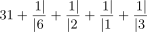
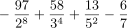

































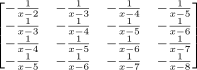










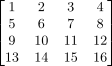
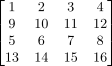


















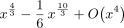





















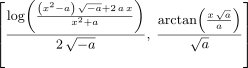



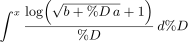


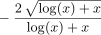









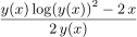










































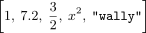


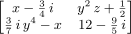
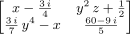
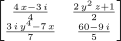
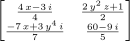
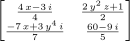
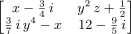
























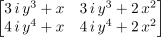












 if no “







 part is optional. The value returned from a conditional expression is
 if the predicate evaluates to
 otherwise. If no



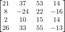


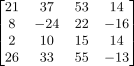










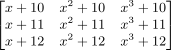














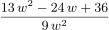


















































 ), and by an expression involving the
parameters, the evaluation of which determines the return value of the function.







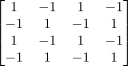



















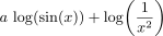



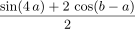


















![[[[1.0, 1.0], [0.0, 1.0]], [[0.0, 1.0], [0.0, 0.0]], [[0.0, 0.0], [1.0, 0.0]], [[1.0, 0.0], [1.0, 1.0]], [[1.0, 0.5], [0.5, 0.0]], [[0.5, 0.0], [0.0, 0.5�](book-2d341a42ef58d325ed073118791429a0.svg)






![[[Hue: 1 Weight: 1.0] from the Pastel palette, [Hue: 1 Weight: 1.0] from the Pastel palette, [Hue: 1 Weight: 1.0] from the Pastel palette, [Hue: 1 Weight: 1.0] from the Pastel palette, [Hue: 14 Weight: 1.0] from the Dim palette, [Hue: 1](book-327b69624561baf84eed8985e7aea770.svg)
![[[Hue: 22 Weight: 1.0] from the Pastel palette, [Hue: 11 Weight: 1.0] from the Light palette, [Hue: 14 Weight: 1.0] from the Dim palette, [Hue: 1 Weight: 1.0] from the Bright palette, [Hue: 14 Weight: 1.0] from the Light palette, [Hue: 11](book-47d08bf6701a4df0c38080eafafee0bf.svg)













































































































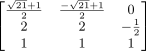


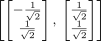





























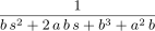


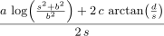

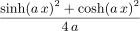
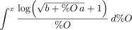
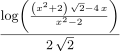



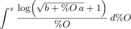

























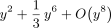



























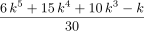







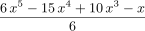
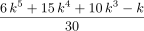
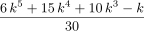






















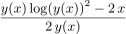



































































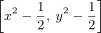





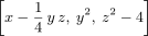





































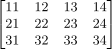


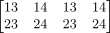


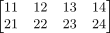

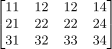

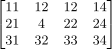


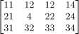



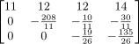


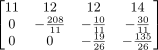
































![[[[1, 2, .], 3, [4, 5, [5, 6, 7]]], 8, .]](book-a0c57a88796942a6d7924836f630a9c2.svg)


![[less= [1, 2, .], greater = [[., 3, [4, 5, [5, 6, 7]]], 8, .]]](book-1f51df15790af295e95b14c6b546f07b.svg)
![[[[1, 2, .], 3, [4, 5, [5, 6, 7]]], 8, .]](book-b42f16578330a7881f6711a1826d767a.svg)












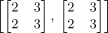
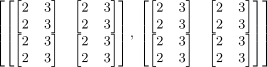

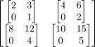





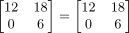
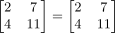
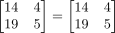
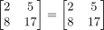
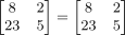
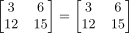
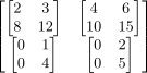
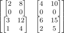
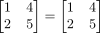
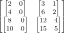


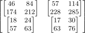

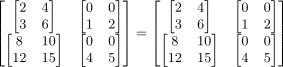



















































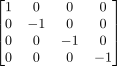
























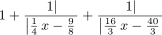






















































































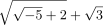
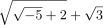

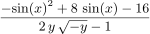













































































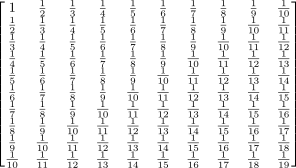







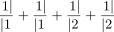
























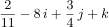






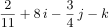


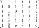












![[[f(n): − f(n+ 3)+ (4 x2− 2n− 4) f(n+ 2)+ ((− 8n− 16) x2+ 4n2 +16n + 16) f(n + 1)+(8n3 +32n2 +40n + 16) f(n)= 0, f(0) =1, f(1)= 4x2, f(2)= 16x4− 16x2+ 4]�](book-14709c4204994bafae19dc97dbe360b0.svg)










































































































































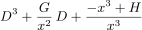


![[[ ( ) ( ) ( ) ( ) &
s0G- 3s0H-+-s0G2+-6s0G- (9s0G-+-54-s0)-H-+s0G3-+-18-s0G2-+-72s0G 27s0H2+--18s0G2-+378s0G-+-1296-s0--H-+s0G4-+-36-s0G3-+-396s0G2+-1296s0G- (135s0G-+-2268-s0) H2-+-30s0G3+-1350s0G2+-16416s0G-+38880s0-H-+-s0G5+-60s0G4-+1188s0G3-+9504s0G2-+25920s0G- 405s0H3 +
s1 = 3 , s2 = 18 , s3 = 162 , s4 = 1944 , s5 = 29160 , s6 = 524880 , s7 =](book-2fdeac046731ae4de7609421f75af0c7.svg)



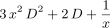


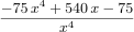






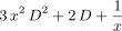











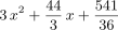







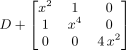
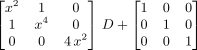





































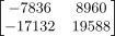
















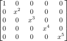
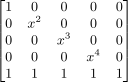
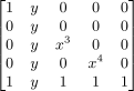
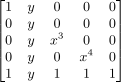

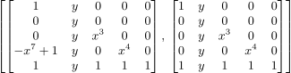

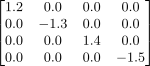

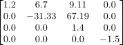
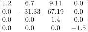


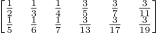

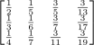


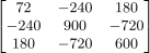
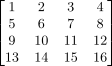

























































































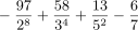

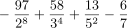


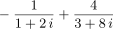
























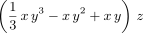




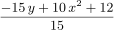


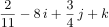








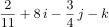





























![[[− 2, − 1[, [− 1, 0[, [0, 1[, [1, 2[]](book-e46bab7d2ec2b282925e9e4947bc6243.svg)









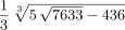
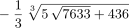















































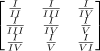
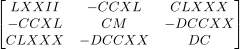










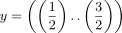














































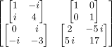
























































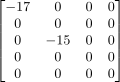


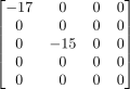
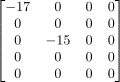





















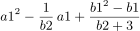




























































































![[[ [ ]] [ [ ]] [ &
complexRoots= ?12 − 12?11+ 24?10+ 4?9− 9?8+ 27 ?7− 21 ?6 +27?5 − 9?4 +4?3 +24?2− 12? +1, coordinates= 63 x+ 62%A11 − 721%A10 + 1220%A9 + 705%A8 − 285%A7 + 1512%A6 − 735%A5 + 1401 %A4 − 21%A3 + 215%A2 + 1577 %A − 142, 63y − 75 %A11+ 890%A10 &#](book-915ea4664c4d7ed4187c26a28e0d1dd5.svg)







![[ [ [
[complexRoots = ?, coordinates= [x− 1, y− 1, z+ 1, t− %A ]], [complexRoots= ?, coordinates= [x, y− 1, z, t− %A ]], [complexRoots= ?− 1, coordinates = [x, y, z, t− %A ]], [complexRoots= ?, coordinates= [x &](book-02c59e6ddfc93d8beead401fd6c21496.svg)

![[[complexRoots= ?4+ 5?3+ 16?2+ 30 ?+ 57, coordinates= [151x+ 15%A3 + 54%A2 +104%A +93, 151y − 10%A3 − 36%A2 − 19%A − 62, 151z− 5%A3 − 18%A2 − 85 %A − 31, 151t− 5%A3 − 18%A2 − 85%A − 31]], [complexRoots = ?4 −](book-16d645a0aa46099533ba5264de1392e1.svg)


















































